
The nonrelativistic Coulomb Hamiltonian fixes exact scale relations once its kinetic and attractive terms are supplied. Those relations test a common operator; they do not independently select its coupling.
Specify the coordinate, operator and dictionary
Use the relative separation r of two constituents and the three-dimensional Hamiltonian H=−D∇²−C/r, with D,C>0. Take its lower-bounded quadratic-form realization on square-integrable wavefunctions. The dissociation threshold is zero. This gives a precise binding question: is there a normalized state below that threshold, and what other quantities does the same state predict?
For physical matching, set D=a²/(2μ), C=gac and μ=meM/(me+M), where a is the action scale. Identifying a with ℏ and g with electromagnetic α is an additional dictionary. The source proposal must retain its clock convention as well, since phases and frequency comparisons use that action scale. Three-dimensional geometry and the Coulomb potential are inputs to this benchmark.
Derive the scale and verify the lower bound
Substitute exp(−r/rB) into the radial equation. Its Laplacian is [rB−2−2/(rrB)] times the same function. Cancellation of the 1/r coefficient fixes rB=2D/C, and the remaining energy is E1=−C²/(4D).
Integration by parts, using ∇·r̂=2/r, proves this identity first on appropriate smooth states and then through the closed form. The exponential saturates it. Thus the calculation establishes the global ground energy, not just a trial-state estimate. A discrete source approximation should approach both the energy and this shape under its declared refinement, with finite-domain and discretization errors separately controlled.
Normalize the state and compare the right probability
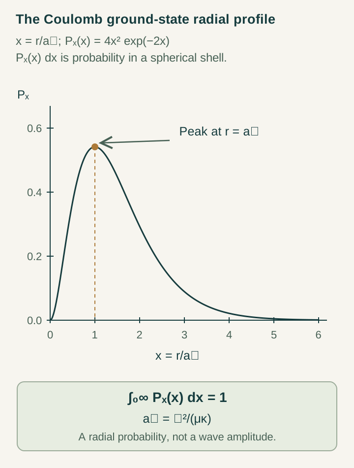
The normalized ground state is ψ1=exp(−r/rB)/√(πrB³). A radial shell has probability density P(r)=4r²exp(−2r/rB)/rB³. Its integral is one; its maximum is at rB; its moments are ⟨r⟩=3rB/2 and ⟨r²⟩=3rB².
Open the full-size diagram →
A comparison must distinguish this radial density from density per unit volume, which peaks at the origin. Neither describes a sharp orbit. The finite moments and normalization give independent numerical checks for a proposed completed spatial record, instead of judging its appearance by a single plotted peak.
Change one coefficient and predict every linked scale
Use the explicit model units D=1/2 and C=1. Then rB=1, E1=−1/2, ⟨r⟩=3/2 and ⟨r²⟩=3. Doubling C while keeping D fixed gives radius 1/2, energy −2, mean separation 3/4 and second moment 3/4. Every result follows from one coefficient change.
These two well-defined models are the comparison pair. Both bind and have the same dimensionless radial curve, so binding and normalized shape do not choose the coupling. Their absolute scales differ: radius scales as C⁻¹ and binding magnitude as C². A model fitted only to one radius must still explain its energy dictionary. Matching separate energy and length scales independently can hide a failure of the shared operator relation.
A particularly useful invariant is |E1|rB²=D. It equals one half in both worked models, even though their radii and energies differ. Once D has been independently fixed by the kinetic dispersion, a radius measurement determines the associated binding energy in this family. Treating D as another separately adjustable atomic parameter would remove that cross-check.
Use relative RMS speed rather than an imagined orbit
The Coulomb virial identity gives 2⟨T⟩=−⟨V⟩ and ⟨T⟩=−En. With T=p²/(2μ) and En=−μc²g²/(2n²), it follows that:
ve,rms/c=(μ/me)g/n
The second expression is the electron speed about the center of mass. It becomes the relative result only for an infinitely heavy nucleus. In the real stationary 1s state the probability current and mean velocity vector are zero, although momentum variance is nonzero. After electromagnetic matching, the ground relative RMS ratio equals α. That is a consequence of the supplied Hamiltonian, not an independent calculation of α from a temporal delay.
Use ratios and cycle identities before fine corrections
The same Coulomb operator has En=E1/n². Writing B=|E1|, its 1→2 interval is 3B/4 and its 2→3 interval is 5B/36, so their ratio is 5/27. A common action convention gives angular frequency ΔE/a and ordinary frequency ΔE/(2πa). Confusing these conventions produces a factor of 2π without any new physics.
All stationary transition frequencies must satisfy ν13=ν12+ν23. These exact checks test a common level model, but they do not determine transition intensities or lifetimes. Spin, relativistic corrections, radiation, recoil beyond reduced mass and nuclear structure require extra operators before comparison with precision atomic measurements.
Turn the benchmarks into a source-level challenge
Freeze the generative update, completion rule and independently matched coefficients before comparing its normalized profile, binding energy, momentum variance and spectral ratios. Count retained failure outcomes if preparation uses a selective filter. High conditional ground fidelity and high preparation probability are separate results; unitary phase evolution alone does not relax an excited state to the ground state.
SMM interprets a bound mode as persistent organization of one source, while DTT places its construction in six nested inner roles and its accessible record at outer completion. A substantive derivation must recover the common effective operator and dictionary from those operations. If it also fixes g upstream, the atomic scales become additional predictions. The isotope comparison then tests whether that same operator gives the different reduced-mass dependences correctly.
When comparing a finite numerical domain, verify that the omitted exponential tail is below the declared error target. For the exact radial state, the probability outside R is e−2R/rB[1+2R/rB+2(R/rB)²]. This gives an analytic boundary benchmark without inventing an experimental accuracy or a source discretization law.
Continue with the articles
- Why the Coulomb law requires a continuum input
The inverse-distance potential follows from a decaying three-dimensional Poisson kernel. The graph-to-continuum limit fixes its geometric form only under stated assumptions, while the physical interaction strength remains a separate matching question.
- A normalizable hydrogen-like ground state
Square completion gives the exact normalized ground state of the supplied nonrelativistic Coulomb Hamiltonian. Its spectrum and relative root-mean-square speed provide precise atomic benchmarks without selecting the coupling itself.
- Completion as ground-state selection
A normalized two-outcome energy filter approaches the ground state along accepted sequences when the initial overlap is nonzero. Its fidelity bound is distinct from preparation yield, radiative relaxation and an autonomous completion mechanism.
- Why binding does not fix the coupling
Dilation shows that every positive Coulomb coupling admits binding and the same type of ground-state filter. A source derivation of a particular coupling must therefore fix field, matter, action and clock normalization beyond the existence of an atom.
- Freeze parameters before predicting spectroscopy
A spectroscopy test becomes predictive when its operator family, coefficients and calibration data are fixed before the reserved transitions are examined. The freeze record makes the dependency between constants and atomic predictions auditable.
- Recovering a QED baseline before adding residuals
A temporal residual can be assessed only after the conventional atomic baseline, shared level energies and correlated uncertainties are controlled. This guide develops transition-cycle checks and a validation sequence for that comparison.