
Inner order describes generation. Outer order concerns completed records. Six nested roles can organize the first, while a completion interface makes the second available. Physical duration requires a specified clock and calibration.
1. Generation, completion, and duration
DTT distinguishes the activity through which a configuration is formed from the completed configuration available for observation. The first role is called inner or generative time; the second concerns outer completion and the succession of accessible records. This distinction asks us to account for the formation of the observable world, including the clocks within it.
Three notions should be kept separate. Order tells us which operation or event precedes another. Completion tells us when an admissible result has been produced. Duration compares an interval with a physical standard. A list of completed events can have an order even when no equal-duration tick has been established.
In a state-update model, an iteration label n tracks applications of a map U. A clock reading T is an observable of the model’s state or records. If T advances uniformly with n in a specified regime, that is a property to demonstrate. If the number of internal operations per completed event varies, event count and duration can also vary independently.
2. Six nested roles and the seventh completion
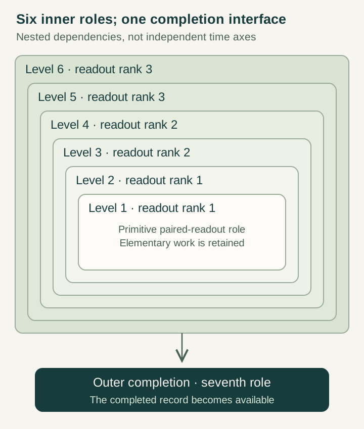
The six inner levels are organized by dependency: a higher stage uses or completes work organized at lower stages. This can be represented by carry periods, composed operations, or successively available records. The seventh role is the interface at which the assembled result becomes a completed observable configuration.
In the paired readout used in several explanatory constructions, the successive ranks are 1, 1, 2, 2, 3, 3. Two roles support one signed direction, then another pair supports a second direction, then the final pair a third. The rank sequence describes that architecture. It is not a list of six independent laboratory clocks, and the outer completion is not a seventh spatial coordinate.
Open the full-size diagram →
The hierarchy can be used in a finite mathematical realization while its physical selection remains a further question. To show necessity, one must identify which source assumptions require the pairing, the allowed primitive channels, and one channel per level. Merely naming six stages does not establish that alternatives are impossible.
3. A counter model with an exact rank calculation
Let q be an integer radix at least 2. Write a single counter in six digits d₁,…,d₆, with the lowest digit changing most often. The higher digits advance after completed lower-digit cycles. This is one update sequence. The six digits advance at intervals q⁰, q¹, …, q⁵ elementary updates; their full return periods are q, q², …, q⁶.
Q(d) = ℓ[(d₁−d₂)e₁ + (d₃−d₄)e₂ + (d₅−d₆)e₃].Q is a supplied spatial readout. The independent vectors e₁,e₂,e₃, their pairing, and the length scale ℓ are inputs to this example.
During the first qᵃ counter addresses, the first a digits vary freely and the remaining digits are zero. The first digit varies along e₁; its partner changes the same coordinate with the opposite sign. The third digit introduces e₂, and the fifth introduces e₃. Hence the affine rank of that prefix is ⌈a/2⌉.
| Available digits | Independent readout directions | Rank |
|---|---|---|
| d₁ | e₁ | 1 |
| d₁,d₂ | e₁ | 1 |
| d₁,…,d₃ | e₁,e₂ | 2 |
| d₁,…,d₄ | e₁,e₂ | 2 |
| d₁,…,d₅ | e₁,e₂,e₃ | 3 |
| d₁,…,d₆ | e₁,e₂,e₃ | 3 |
The derivation is exact for this map. It exhibits how nested work can open successively higher-rank records. Because the three-direction frame was supplied in Q, it is not a proof that an unstructured source selects three-dimensional physical space. The selection problem asks why an appropriate map and stable local relations should follow from the source dynamics.
4. The binary example: 64 addresses, 27 sites
Set q = 2. Each digit is either zero or one, so the source counter has 2⁶ = 64 addresses. Each paired difference can take the values −1, 0, or 1. The completed readout therefore has 3³ = 27 distinct sites in the chosen frame.
A zero difference has two representations, (0,0) and (1,1), whereas +1 and −1 each have one. Across three pairs, the central site has 2³ = 8 source addresses, while a corner has one. Uniform visitation of addresses consequently does not produce a uniform probability over sites.
Why this matters
A record rule might retain the multiplicity, average over it, or choose one representative per site. Those choices give different observable statistics. A proposed spatial measure therefore needs its own derivation; a picture of 27 regularly arranged sites does not determine it.
The counter’s private scan also need not represent a particle trajectory. Carry operations can reset several digits and make large jumps in Q. Physical transport requires a law for propagation between retained records, together with a clock and a bound on the allowed influence. Generation order and matter motion should be connected through that law rather than identified by their labels.
5. What makes a return a completion?
A phase may return to its starting point without any result having been formed. To use recurrence as a completion marker, the model must connect the phase root to a certificate that the record is ready. In a simple notation, κ(z) = 1 marks completion and φ(z) = o marks the selected phase root. The desired compatibility is that these conditions agree on the relevant states.
A finite verification stage can check a parity condition, consistency relation, or return to a designated interface. A quantum description may use a completion instrument with accepted, rejected, and incomplete outcomes. The state changes associated with those outcomes and their probabilities belong to the model. Looking only at successful records can hide both a resource cost and a selection effect.
The outer role becomes meaningful when this mechanism makes the completed result accessible and retained. It can organize a record sequence without assuming that an observer directly measures every internal operation.
6. From record order to a clock
Assigning positive delays to allowed advances can turn a record sequence into a numerical timing model. For composed advances, a natural condition is additivity. For a global event-time function, one needs the delay of an advance to be a difference of event values.
ΔT(a) = T(target a) − T(source a).Additivity and an exact event-time assignment are distinct requirements. Positive delays around a directed cycle obstruct such a global assignment.
If every nontrivial allowed advance has strictly positive exact delay, two distinct events cannot each be later than the other. Otherwise adding the two positive delays would give a positive total for a return to the same event, contradicting exactness. This is a short route from a clock condition to an acyclic event order.
Physical calibration remains necessary. The scale of T must be linked to a repeatable process, and the same law should account for how clocks respond to the relevant source operations. A clock that ignores branch-generation activity and a clock that accumulates it can assign different durations to the same completed configuration. The clock-independence article and the joint clock–band construction explore this issue.
7. Ordinary complex phase and split-complex geometry
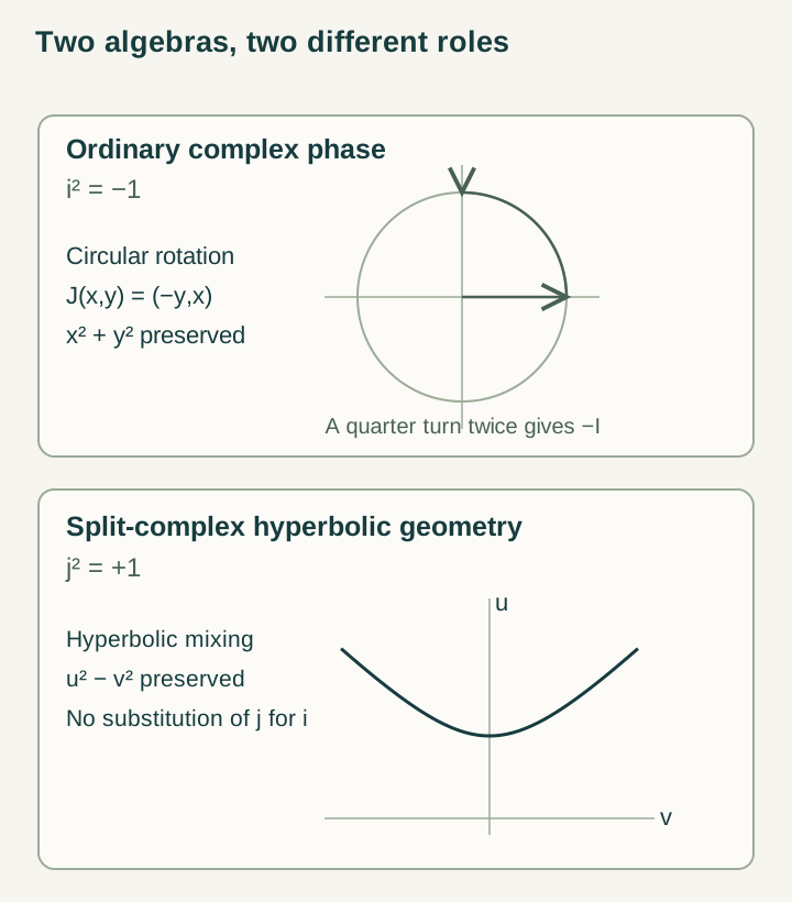
Two different algebras appear in discussions of DTT. Ordinary complex numbers use i² = −1 and describe circular phase rotations. Split-complex numbers use j² = +1 and support a hyperbolic quadratic form. Their similar notation can hide an important distinction.
ejη = cosh η + j sinh η, j² = +1.
For z = u + jv, multiplication by eʲη gives u′ = u cosh η + v sinh η and v′ = u sinh η + v cosh η. Substitution verifies u′² − v′² = u² − v². This algebra realizes a one-plus-one-dimensional hyperbolic transformation. Connecting u and v to physical clock and displacement measurements requires a separate interpretation and unit convention.
Open the full-size diagram →
In real-Hilbert phase selection, the imaginary unit is represented by an operator J satisfying J² = −I. Under appropriate assumptions it can be selected from an oriented real generator. That construction and the split-complex hyperbolic description address different mathematical tasks. A physical theory must specify their common origin or their interface rather than interchange i and j.
8. Why recurrence alone does not choose a future
Let a reversible group G act on a phase space and choose a root o. The returns H = {g : g·o = o} form a subgroup. In particular, if g returns to o, so does g⁻¹. A rule that checks only return to the root therefore accepts both orientations. Recurrence supplies repetition, but not a one-sided arrow.
An ordered availability of records can add the missing asymmetry. If a completed operation preserves or increases what an observer can retain and access, it can count as a forward advance. Its inverse may remove available records and therefore fail that condition. The observable forward operations can form a monoid even when the underlying reversible returns form a group.
The origin of the asymmetry is then explicit: a preparation, a memory mechanism, an access restriction, or a boundary condition. A record arrow is not automatically a thermodynamic entropy theorem. To establish entropy production, the model must specify states, probabilities, the chosen entropy, and an appropriate balance or monotonicity argument.
9. A short derivation of memory after projection
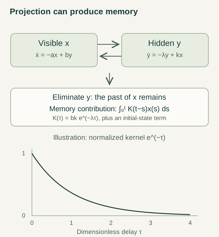
A reduced observer can experience history dependence even when the larger system has local first-order equations. Let x be visible and y a hidden relaxation mode, with λ > 0. Consider the supplied linear model below.
y(t) = e−λty(0) + k∫₀ᵗ e−λ(t−s)x(s) ds.
ẋ(t) = −a x(t) + b e−λty(0) + bk∫₀ᵗ e−λ(t−s)x(s) ds.
The second line follows by multiplying the y equation by eλt and integrating; substituting into the x equation gives the third line. The memory kernel is K(τ) = bk e−λτ. The initial hidden state contributes a separate transient. Thus eliminating y has not made its effects disappear: they enter through the past of x and the hidden initial condition.
Open the full-size diagram →
Memory alone does not establish dissipation. For a > 0 and λ > 0, the two-variable system is asymptotically stable when aλ − bk > 0; that condition follows from the trace and determinant of its evolution matrix. An entropy law would require additional structure. The calculation instead demonstrates the precise DTT-relevant distinction between the complete generative state and the smaller visible state.
10. Reading different DTT formulations together
The published temporal-asymmetry work uses two coupled temporal parameters and a projection to observable evolution. The newer same-cycle and nested-stage formulations seek a more restrictive organization in which generative activity and completed records are roles of one source process. These formulations share a motivation, but their variables and assumptions must be translated explicitly.
A theorem for a two-parameter manifold cannot automatically be imported into a one-counter model. Conversely, the nested counter example does not establish the full connection or curvature structure of the published model. A careful comparison identifies the state space, the evolution law, the completion map, and the observables on each side.
That comparison is productive: it identifies which ideas are reusable and which additional result would unify them. The temporal-asymmetry paper guide develops the reduction viewpoint, while the postulate guide below gives a compact checklist for a concrete source model.
Further reading
Continue with the individual articles and their source references.
- One action, two temporal roles
Inner generation and outer record order can be roles of one process. A completed return becomes an observable advance only when its action respects the retained records and their tests.
- Why recurrence alone does not select a future
Reversible recurrence admits both a return and its inverse, so a phase root alone cannot select the future. An observable arrow needs additional record, preparation, or clock structure.
- From available records to a temporal arrow
Completed returns that preserve or increase accessible records form a positive monoid. Under additional separation and clock conditions, this supplies an effective forward order without proving thermodynamic irreversibility.
- When an additive clock is unique
An ordered rank-one return structure permits a faithful additive scalar clock only up to positive rescaling. Independent return directions and path-dependent delays show where that uniqueness stops.
- Nested operations and clock independence
Clock independence must survive every admitted interleaving of branch and resolution operations. The orbit-algebra criterion removes branch effects from all such finite sequences and supplies an accumulated-error bound.
- From record refinement to a joint clock–band relation
Independent count, scale, phase, clock, and band measurements can satisfy a joint refinement relation under the supplied interfaces. The ungated-clock alternative identifies why the protected-clock premise remains essential.
- Six inner stages and one publication interface
A six-digit nested counter with paired signed readout realizes ranks 1, 1, 2, 2, 3, 3 before one completion interface. Its exact counts reveal sampling bias and the restricted assumptions behind the six-channel bound.
- What spatial readout forgets
Different inner states can share one spatial readout and still have different successors. A concrete counterexample and a kernel-preservation criterion identify the memory needed for autonomous completed evolution.
- Real-commutant phase selection: a paper guide
An oriented real orthogonal flow can select an ordinary complex structure on its dynamic sector. Planar examples explain residual zero-mode freedom, time-reversal antilinearity and the extra balancing rule needed for composite systems.
- Temporal asymmetry: reading the published model
The temporal-asymmetry model connects projected dynamics with memory and path dependence. A solvable hidden-mode example distinguishes those effects from dissipative stability and from evidence for a second observable clock.
Continue the connection
Follow the next guide, or return to the reading paths.