
For H=−DΔ−C/r with D,C>0, square completion proves E₁=−C²/(4D) and the normalized exponential ground state. Its SMM/DTT role is a precise target for generated matter dynamics.
State the atomic problem completely
Use the relative separation r between two constituents in three-dimensional space. The effective Hamiltonian is H=−DΔ−C/r, with positive coefficients D and C. The state space is square-integrable complex wavefunctions, and the operator is understood through its lower-bounded quadratic form and the corresponding Friedrichs realization. The separation threshold is zero in this convention.
The model assumes continuum geometry, coherent kinetic evolution, and an attractive Coulomb potential. Its immediate question is whether these ingredients produce a normalized localized state below threshold. For SMM/DTT this isolates a concrete completion target before introducing spin, radiation, or nuclear structure.
Find the scale through direct substitution
A negative-energy localized state should decay at large r. Try ψ proportional to exp(−r/a). For this radial function, Δψ=(a−2−2/(ar))ψ. Acting with H gives a constant term −D/a² and a term proportional to (2D/a−C)/r. Choosing a=2D/C cancels the variable term exactly.
This finds an eigenstate and its energy. To show that it is the ground state rather than one among many negative-energy states, a lower bound for arbitrary admissible wavefunctions is still required.
Prove the global lower bound
Expand the squared norm of ∇ψ+r̂ψ/aB and integrate the cross term by parts. The identity ∇·r̂=2/r produces exactly the attractive Coulomb term when aB=2D/C. Initially this can be checked on suitable smooth functions, then extended through the closed quadratic form.
Every normalized state therefore has energy at least −D/aB². The exponential makes the integrand vanish and saturates the bound. This proves the stated ground energy, rather than relying on an uncertain classical orbit or a variational guess.
Normalize the state and read the figure correctly
The normalized state is ψ1(r)=exp(−r/aB)/√(πaB³). Its density per unit volume is largest at the origin. The probability per radial interval includes the spherical-shell volume, giving P(r)=4r²exp(−2r/aB)/aB³. This function is largest at r=aB.
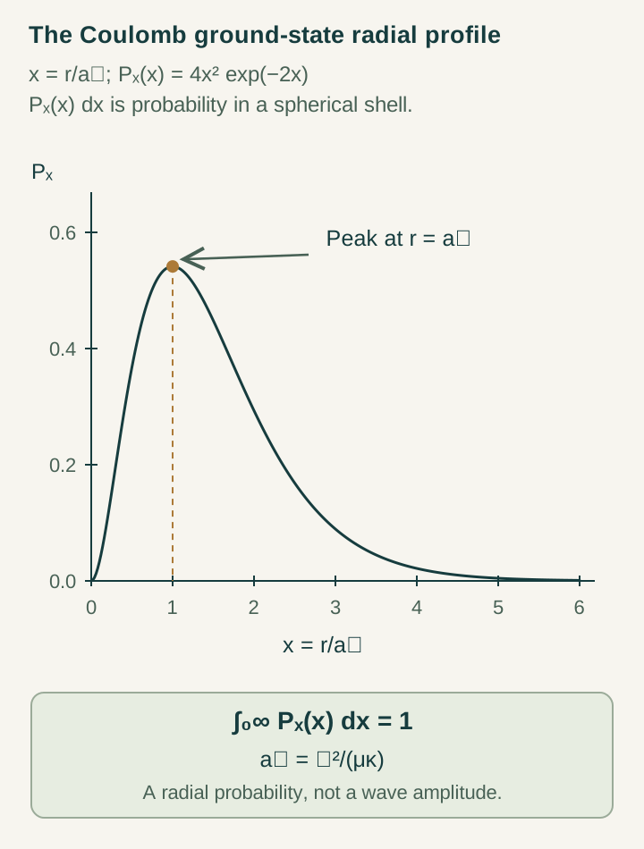
Open the full-size diagram →
A radial probability peak does not describe an electron moving around a circular track of that radius. The real stationary ground wavefunction has zero probability current. Its nonzero momentum variance expresses a different observable, developed in the alpha-and-motion guide.
The spatial spread can also be checked exactly. Integrating the same radial density gives ⟨r²⟩=3aB² and hence a radial standard deviation √3aB/2. The spread is comparable to the characteristic radius; localization means a normalizable distribution with finite moments, not a sharply fixed separation. These moments are useful independent checks for a numerical state produced by a proposed discrete source model.
Worked example and the bound spectrum
Set D=1/2 and C=1 in model units. Then aB=1, E1=−1/2, and P(r)=4r²e−2r. The state is normalizable and lies below the separation threshold. The exact excited energies are En=−1/(2n²); separating the radial equation gives n=nr+ℓ+1.
The gap from n=1 to n=2 is 3/8, and the gap from n=2 to n=3 is 5/72. Their ratio is 5/27. This scale-free check tests the supplied Coulomb spectral structure. It does not determine the overall energy unit, line intensity, or spontaneous-emission lifetime, which require additional physical input.
Introduce mass, action, and coupling
For an electron of mass me and nucleus of mass M, separation of center-of-mass motion gives reduced mass μ=meM/(me+M). Set D=ħ²/(2μ) and C=għc. The model then has aB=ħ/(μcg) and En=−μc²g²/(2n²). Electromagnetic matching identifies g with α.
The reduced mass belongs to the relative coordinate, not to a redefinition of the electron’s intrinsic mass. Also, the atomic formulas do not determine g: changing a positive g changes the size and binding energy while preserving the dimensionless state shape. The source must independently select the response normalization to derive a coupling.
The spinless level multiplicity is n² before additional internal degrees of freedom are included. Adding an electron spin label changes the state bookkeeping; deriving the associated magnetic and relativistic responses requires new operators, not just doubling that count.
A stable completed mode with evolving phase
Under outer evolution exp(−iHT/ħ), the ground mode acquires a phase while its density remains stationary. This makes temporal resonance a precise description of the supplied model. Observable transition beats depend on energy differences, so changing the overall energy reference does not change the spectral predictions.
The SMM/DTT challenge is to obtain this operator and its dictionary from nested inner generation. A successful source model should reproduce the lower bound, exponential profile, shared scale relations, and excited spectrum together. These linked benchmarks prevent a model from fitting the radius while leaving the energy or probability rule unexplained, and provide a disciplined starting point for spin and radiative structure.
Continue with the articles
- A neutral pair is not yet an atom
Charge neutrality does not establish an atom: binding requires a localized state below a defined dissociation threshold. A minimal Coulomb example separates that requirement from finite-box gaps, classical orbit pictures and source-level selection.
- Why the Coulomb law requires a continuum input
The inverse-distance potential follows from a decaying three-dimensional Poisson kernel. The graph-to-continuum limit fixes its geometric form only under stated assumptions, while the physical interaction strength remains a separate matching question.
- A normalizable hydrogen-like ground state
Square completion gives the exact normalized ground state of the supplied nonrelativistic Coulomb Hamiltonian. Its spectrum and relative root-mean-square speed provide precise atomic benchmarks without selecting the coupling itself.
- Why binding does not fix the coupling
Dilation shows that every positive Coulomb coupling admits binding and the same type of ground-state filter. A source derivation of a particular coupling must therefore fix field, matter, action and clock normalization beyond the existence of an atom.
- Hydrogen fine structure and its temporal interpretation
The standard fine-structure Hamiltonian gives a quantitative benchmark for a temporal account of spin and relativistic transport. Its shared coefficients and n=2 splitting specify what a source model must reproduce before proposing additional shifts.