Completion as a controlled ground-state selection

Ask how the persistent record is reached

A Hamiltonian can possess a stable ground mode without driving every initial state into it. Under isolated unitary evolution, the probabilities of energy eigenstates remain fixed. To explain preparation, a theory must include an interaction with other degrees of freedom, a selective measurement, or another explicit open-system mechanism.

In DTT, outer completion motivates a distinction between generative histories and accepted observable records. A mathematical instrument makes that distinction precise: it specifies outcomes, their probabilities, and the corresponding state changes. The construction below is a controlled preparation model, not an assertion that all isolated atoms undergo a new universal collapse law.

Build the acceptance and rejection operators

Let H have ground energy E₀ and H−E₀≥0. For s>0, define K_s=exp[−s(H−E₀)]. Its eigenvalues lie between zero and one, so it is a contraction. The parameter s has units of inverse energy; a laboratory duration requires an additional implementation.

For density operator ρ, acceptance has probability tr(K_sρK_s), with conditional state K_sρK_s divided by that probability. The rejection operator supplies the complementary branch, ensuring total probability one.

Derive the fidelity bound

Assume a unique normalized ground state ψ₀ and gap Δ>0 to the rest of the spectrum. Write ψ=√p ψ₀+χ with χ orthogonal to ψ₀, where 0<p≤1 and ‖χ‖²=1−p. The filter leaves the ground component unchanged and shrinks the excited component by at least e^−sΔ in norm.

Here m is the number of consecutive accepted applications. The bound follows by dividing the residual excited norm by the accepted total norm, which is at least p. If p=0, this filter cannot create a ground component: improving existing overlap is its mechanism.

Worked example: fidelity and yield together

Choose p=1/4, sΔ=1, and three accepted applications. The infidelity is at most 3e⁻⁶≈0.00744. If the whole excited component lies exactly at energy E₀+Δ, the accepted-sequence probability is P₃=1/4+(3/4)e⁻⁶≈0.25186, and its exact ground fidelity is (1/4)/P₃≈0.99262.

As the number of accepted applications grows, fidelity approaches one while total sequence probability approaches 1/4. The accepted output becomes excellent, but most input trials do not pass the complete sequence. Reporting only the conditional quality would conceal a major part of the preparation behavior.

A measurement register realizes the probability structure

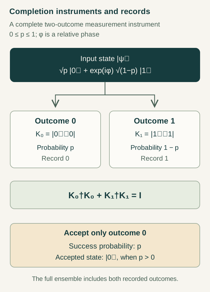
Introduce orthogonal outcome labels |accept⟩ and |reject⟩. The map ψ↦K_sψ⊗|accept⟩+R_sψ⊗|reject⟩ preserves inner products because the two operator squares sum to I. It is therefore an isometry, providing an abstract realization of the instrument with an outcome register.

This construction shows compatibility with quantum measurement mathematics. It does not yet explain how local operations implement the global function of H, how the register is initialized, or how rejection is handled. Resetting a failed trial and retaining its old state are different protocols and must not be treated as interchangeable.

In particular, R_s annihilates the exact ground component because its eigenvalue there is zero. Continuing with the rejected state therefore differs sharply from preparing a fresh input with ground overlap p. A repeated-attempt model needs an explicit restoration operation before assigning the same success probability to every trial.

Apply the same construction to the atom

For the scalar Coulomb Hamiltonian H=−DΔ−C/r, the ground energy is −C²/(4D) and the first excited energy is one quarter of that value. The gap is therefore Δ=3C²/(16D). The same operator that creates binding also sets the filtering scale, which links localization and preparation within this declared model.

Physical atomic relaxation, however, involves radiation, selection rules, energy conservation, and environmental coupling. The filter is not a derivation of spontaneous-emission rates. A dynamical completion mechanism should explain where rejected energy and information go and how its preparation time compares with measurable atomic timescales.

Make completion an autonomous process

The next SMM/DTT step is to replace the abstract instrument with explicit local source operations and retained memory. The six nested inner roles should build the candidate state and comparison apparatus; the seventh role should expose an outcome through a defined record. The same update should determine the observable clock cost.

A useful theorem would bound three quantities together: accepted-state error, acceptance probability, and the resource or duration required to approximate K_s. That would convert completion from a vocabulary for selecting successful histories into a physical preparation mechanism. The spectral construction already supplies a precise target and makes clear which information an autonomous implementation must preserve.

Continue with the articles

• Completion as ground-state selection

  A normalized two-outcome energy filter approaches the ground state along accepted sequences when the initial overlap is nonzero. Its fidelity bound is distinct from preparation yield, radiative relaxation and an autonomous completion mechanism.

• A protected gap in the finite singlet model

  The finite singlet-loop Hamiltonian has a unique ground state and a uniform lower bound on its excitation gap. The derivation identifies the supplied penalty, carrier rank and limits that separate this result from a continuum gauge-theory mass gap.

• A normalizable hydrogen-like ground state

  Square completion gives the exact normalized ground state of the supplied nonrelativistic Coulomb Hamiltonian. Its spectrum and relative root-mean-square speed provide precise atomic benchmarks without selecting the coupling itself.

• Local stability versus the global minimum

  Local stability and global selection occur at different deformation thresholds in the finite SU(2) model. Explicit examples distinguish metastability from energetic preference and show why physical completion also requires dynamics and error control.