
Coulomb and fine-structure calculations supply quantitative baselines. A source-derived correction must enter through compatible level operators, with fixed coefficients and a correlated pattern across reserved transitions.
Begin with one common set of levels
Label each stationary state a by its quantum numbers and assign an energy Ea. The signed transition frequency is νab=(Eb−Ea)/h. This definition immediately imposes a consistency law: νac=νab+νbc. Any proposed temporal correction to stationary spectroscopy must obey the same law.
SMM’s common-source ambition makes this constraint especially useful. Inner histories may differ between states, but their outer completion must produce one compatible energy structure. Independent offsets assigned to each spectral line can destroy that structure even when individual numbers appear plausible.
Recover the leading spectrum first
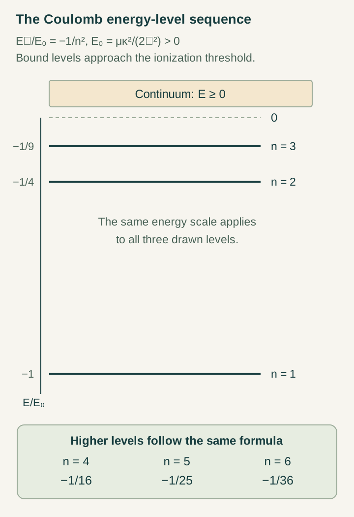
For the nonrelativistic Coulomb operator, En=−B/n², with B=μc²α²/2 after physical matching. The energies approach the zero continuum threshold. Adjacent spacing is B(2n+1)/[n²(n+1)²], approaching 2B/n³ at large n. These are exact consequences of the supplied scalar model.
Open the full-size diagram →
For a worked scale-free check, the 1→2 interval is 3B/4 and the 2→3 interval is 5B/36, giving ratio 5/27. A source construction that recovers this ratio has reproduced part of the Coulomb operator’s structure; it has not thereby fixed B or derived radiative corrections.
Fine structure links spin and motion
In the point-nucleus, infinite-nuclear-mass Dirac–Coulomb benchmark, the leading correction is δEfs(n,j)=−[mc²α⁴/(2n⁴)][n/(j+1/2)−3/4]. The α⁴ scale follows because typical bound momentum is of order mcα, so the relativistic kinetic correction p⁴/(m³c²) has that energy order.
At n=2, the bracket is 5/4 for j=1/2 and 1/4 for j=3/2. Their energy difference at this order is mc²α⁴/32. Correct spin-orbit and contact coefficients are needed to obtain the combined pattern. Reduced mass alone does not supply every recoil correction, and nuclear, radiative, and external-field effects enter later.
An explicit way inner modes can shift levels
Let P select retained atomic states and Q=I−P select auxiliary states of one self-adjoint Hamiltonian. Eliminating the Q component of the stationary equation gives Heff(E)=PHP+PHQ(E−QHQ)−1QHP whenever the resolvent exists. This displays how unresolved generative structure can leave an energy-dependent response in completed records.
For one retained level E0, one auxiliary level E0+Δ, and coupling v, the lower exact energy is E0+Δ/2−√(Δ²/4+v²). At |v|≪Δ its shift is −v²/Δ+O(v⁴/Δ³). This is a calculable auxiliary response. A radiative field loop additionally needs its field states, symmetry constraints, regulator, and matching prescription.
Worked example: one operator, several lines
As a first-order effective insertion, take δH=λδ³(r). It shifts nS states by K/n³, where K=λ/(πaB³), while states with nonzero orbital angular momentum have zero contact matrix element at this order. The delta is used here as a perturbative insertion, not an unregularized standalone three-dimensional Hamiltonian.
The ratio is fixed before λ is chosen. It is a useful cross-state consequence, although ordinary nuclear short-distance effects can share contact-like behavior. Other angular or isotope channels are needed to identify an origin.
Keep the baseline and new operator consistent
A Lamb-shift comparison requires a specified reference containing the relevant self-energy, vacuum-polarization, recoil, nuclear, and higher-order terms. A missing conventional contribution is not a new DTT effect. Likewise, a holonomy phase needs an energy map: a dimensionless cycle fraction alone cannot be subtracted from a measured frequency.
Calculate any proposed correction from a common operator δH=ΣckOk. For nondegenerate levels its first-order shifts are the corresponding expectation values; within a degenerate subspace, diagonalize the perturbation first. This procedure enforces level compatibility and shows which coefficients are independently fixed, fitted, or still unknown.
For a simple holonomy-based example, assign three dimensionless state fractions η1=0, η2=ε, and η3=0 with one shared energy map δEa=Kηa. The first transition shifts by Kε/h, the next by −Kε/h, and the direct 1→3 shift vanishes. The cycle closes automatically. Separate transition-dependent multipliers would generally lose this constraint.
Freeze shared inputs and use complementary channels
Define the calibration set before selecting reserved predictions. A transition already used indirectly to determine a mass, radius, or frequency scale cannot simultaneously count as independent confirmation. Shared uncertainties produce covariance: two lines involving the same level or parameter are generally correlated. A transition network with q connected levels contains only q−1 independent stationary energy differences.
The theoretical priority is to derive an operator relation from the six nested inner roles and one completion law. Hydrogen, isotope variation, and high-angular-momentum states can then test distinct consequences of that relation. A successful result would organize many levels with fewer independent coefficients, making the common source explanatory rather than a separate label attached to each spectral correction.
Continue with the articles
- Hydrogen fine structure and its temporal interpretation
The standard fine-structure Hamiltonian gives a quantitative benchmark for a temporal account of spin and relativistic transport. Its shared coefficients and n=2 splitting specify what a source model must reproduce before proposing additional shifts.
- The Lamb shift as a demanding benchmark
A Lamb-shift calculation requires a defined baseline, regulated interactions and correlated state-dependent coefficients. A first-order contact example illustrates the structure of a test without claiming a computed DTT radiative correction.
- Radiative inner-time loops: defining the proposal
Source recurrence, transport holonomy and a radiative field loop are distinct constructions. An explicit retained-and-auxiliary model shows how resolvent elimination produces an energy shift and what further structure a radiative proposal needs.
- Freeze parameters before predicting spectroscopy
A spectroscopy test becomes predictive when its operator family, coefficients and calibration data are fixed before the reserved transitions are examined. The freeze record makes the dependency between constants and atomic predictions auditable.
- Recovering a QED baseline before adding residuals
A temporal residual can be assessed only after the conventional atomic baseline, shared level energies and correlated uncertainties are controlled. This guide develops transition-cycle checks and a validation sequence for that comparison.
- What would count as a DTT spectroscopic residual?
A DTT spectroscopic residual requires a restricted source-derived pattern across shared atomic levels. A contact example gives a cross-transition ratio while exposing how conventional nuisance effects can imitate the same signal.
- State-dependent record cycles in hydrogen
A state-dependent record cycle needs a specified transport, physical band, phase convention and energy map. Shared level shifts then enforce transition-cycle consistency, which a separate adjustable phase for each line can violate.
- Differential spectroscopy as a test strategy
Differential spectroscopy tests shared state dependence by combining several transitions with a fixed baseline. Contact examples and transition-graph identities show why covariance and independent sensitivity directions matter more than the raw number of lines.
- Hydrogen and deuterium as complementary probes
Hydrogen and deuterium separate universal electronic rules from isotope-specific mass and nuclear effects. Reduced-mass and contact-scaling examples show why a common operator can still produce different numerical shifts in the two atoms.
- Rydberg states and long record cycles
Highly excited states extend the test to larger spatial scales and complementary angular channels. Standard Coulomb scaling and contact-term null channels define what a proposed long-record-cycle correction must calculate independently.
- Designing an overconstrained atomic test
An overconstrained atomic test compares independent residual directions with a declared set of source and nuisance coefficients. Covariance weighting and singular-value analysis reveal whether the chosen observables can actually distinguish the proposed mechanism.