A temporal residual can be assessed only after the conventional atomic baseline, shared level energies and correlated uncertainties are controlled. This guide develops transition-cycle checks and a validation sequence for that comparison.
A residual is meaningful only relative to a sufficiently complete reference calculation. If a candidate SMM/DTT model reproduces the leading Coulomb spectrum but omits an ordinary radiative or nuclear correction, the difference from experiment does not identify new temporal physics. Paper 13 therefore places baseline recovery before additional residuals. The task is to compute the same measured observable under a clearly stated conventional theory, with independently specified inputs and uncertainty. That reference can then be compared with a reconstructed or modified source model in a controlled way.
02Organize corrections by physical origin
Begin with the gross-structure energy and its mass convention. Add relativistic and spin terms, self-energy and vacuum-polarization terms, recoil, finite nuclear size and other nuclear structure contributions at the required accuracy. Hyperfine splitting must be included or removed through an explicitly defined centroid. External magnetic and electric fields alter measured transition frequencies and belong in the measurement model. This organization does not mean all contributions can always be treated independently; mixed corrections occur. The purpose is to identify which term is included at which order and prevent double counting.
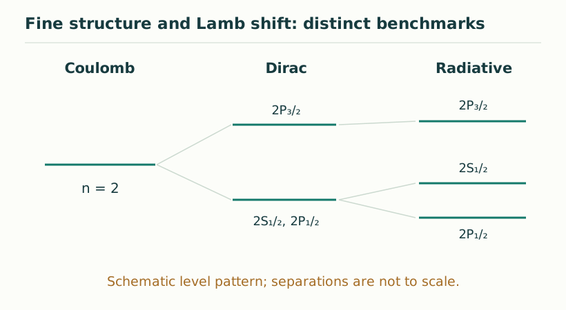
Figure 1. Fine structure and Lamb shift: distinct benchmarks. Schematic only, with deliberately exaggerated separations. For hydrogen n = 2, Dirac fine structure separates j = 1/2 from j = 3/2; radiative corrections further separate 2S₁/₂ and 2P₁/₂. No measured scale is plotted. View full size ↗
03A level-based accounting identity
Write each level as a sum of a reference energy and defined corrections. The transition frequency is the difference of the complete levels divided by h. If a parameter appears in several levels, its uncertainty is shared. A sign error in one level can produce correlated transition discrepancies that resemble a new effect. Constructing levels first supplies a valuable internal check: the oriented frequencies around any closed three-level cycle sum to zero. This identity follows from energy differences and holds regardless of the detailed source interpretation.
Ea = Eref,a + Σk δEk,a; νab=(Eb−Ea)/h.
νac = νab + νbc.
04Why covariance matters
Two transitions sharing a level or an input parameter are not generally independent. If a common constant shifts both predictions, its error moves them together. A covariance matrix records this structure. In linear propagation, parameter covariance Cθ contributes J Cθ Jᵀ, where J contains derivatives of the predicted frequencies. Experimental covariance and declared theory uncertainties must then be included consistently. Treating all lines as independent can exaggerate the significance of a pattern. Conversely, a suitable differential combination can cancel a common uncertainty and expose a smaller effect.
Σparameter = J Cθ Jᵀ; Jab = ∂νa/∂θb.
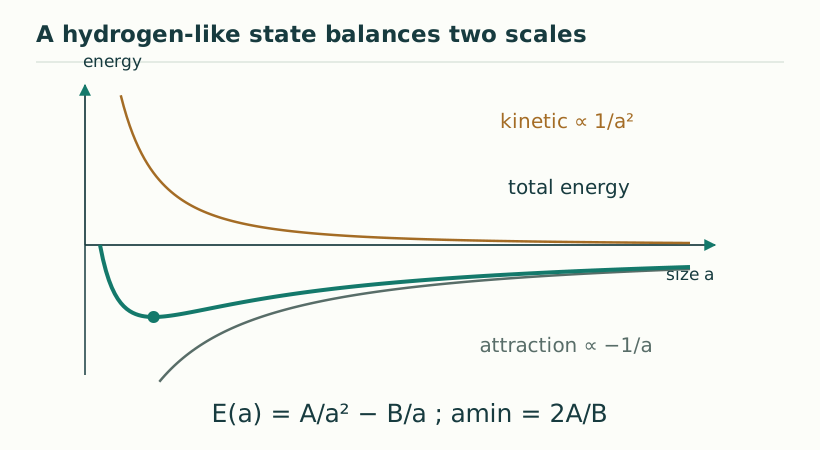
Figure 2. A hydrogen-like state balances two scales. The illustrative variational form E(a) = A/a² − B/a has a minimum at a = 2A/B for A,B > 0. Binding follows once kinetic and attractive terms are supplied; this calculation leaves B, and hence the coupling, free. View full size ↗
05The SMM/DTT reconstruction question
There are two distinct accomplishments to seek. One is to recover the conventional effective operators from inner-generation and outer-completion dynamics, explaining why their coefficients agree. The other is to derive an additional operator with a distinguishable residual pattern. Recovering the first should not be reported as detecting the second. A common generative source is most informative when it constrains several terms together. For example, the same retained phase structure might restrict spin response and field coupling; a paper should prove that restriction and then match it to the baseline rather than assume both coefficients separately.
06Cancellation can amplify numerical error
Suppose a target interval is the difference of two large calculated levels. Correctly evaluating each level to many relative digits does not automatically give the small difference to the desired absolute accuracy. If the separate numerical errors are εa and εb, the interval error is (εb−εa)/h and can dominate a tiny residual. Shared analytic terms should be canceled symbolically where possible, and the remaining calculation should be tested by increasing numerical precision or tightening a specific convergence parameter. The same issue occurs when extracting a new temporal contribution from a much larger baseline. Displayed decimal places should reflect the propagated interval uncertainty, not the precision of an intermediate energy value.
07A useful validation ladder
First verify the analytic limiting cases of the model. Then compare its numerical level solver with known exact Coulomb and point-nucleus Dirac limits. Next add corrections with units and signs checked separately, and verify transition additivity. Finally propagate correlated uncertainties and compare reserved observables. The uncertainty target should determine the truncation order, not the desire to display many decimal places. A discrepancy larger than numerical error but smaller than an omitted conventional term is not evidence of a DTT effect. Keeping the uncertainty budget at each stage makes it possible to identify which approximation limits the final comparison.
KEEP THE CONNECTION
Key ideas
A residual depends on the completeness and convention of its baseline.
Build shared levels before forming transition frequencies.
Correlated uncertainties and omitted corrections must be controlled.
Scope of the argument. Methodology for a future comparison, with standard baseline structure; no new residual is inferred from data.
Sources & further reading
Temporal Reconstruction of Hydrogen III, skeleton research outlinepaper13_hydrogen_fine_structure_lamb_shift.pdf, §§2–7, pp.3–9
Minimal hydrogen note: transition consistency and contact correctionsmm_dtt_minimal_hydrogen.pdf, §8.1, p.7
Temporal Reconstruction of Hydrogen III: Fine Structure, Lamb Shift, and Radiative Inner-Time Loops
Working manuscript. Article-level references identify the consulted sections and the scope of the interpretation. No public URL was supplied for this exact manuscript version.