
A shared coupling produces energies proportional to reduced mass, radii inversely proportional to it, and a shared contact insertion proportional to its cube. These distinct scalings constrain a common source model without assigning a DTT residual.
Derive the leading mass ratio explicitly
Separation of center-of-mass motion gives μ=meM/(me+M). Use illustrative inputs MA=1000me and MB=2000me; these are chosen model masses, not measured nuclear masses. Then μA/me=1000/1001 and μB/me=2000/2001.
At fixed g, each Coulomb transition energy in B is q times its counterpart in A, while each characteristic radius is 1/q times as large. Thus the fractional leading energy difference is exactly 1/2001 in this toy comparison. No new temporal effect is needed: the ordinary two-body Hamiltonian already predicts a nonzero isotope shift. The mass convention must be fixed before defining any residual.
Check several observables against the same mass change
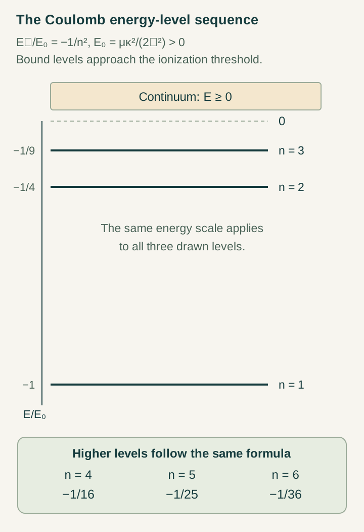
The leading levels are En=−μc²g²/(2n²), the Coulomb length is rB=a/(μcg), and the relative RMS speed is cg/n. Consequently the first two depend on μ, while the relative RMS speed does not. Electron center-of-mass RMS speed does change, through μ/me.
Open the full-size diagram →
The figure shows exact dimensionless level ratios shared by the two model isotopes, not measured isotope splittings. Each isotope retains the interval ratio 5/27 between 2→3 and 1→2. Rescaling an entire energy diagram cannot by itself test a new source law; the stronger comparison checks the distinct radius, energy and velocity dependencies using one unchanged interaction and clock convention.
Compute a different mass dependence for a contact insertion
As a first-order comparison operator, take δH=λδ³(r) with one shared coefficient λ. It is an effective perturbative insertion, not an unregularized standalone three-dimensional Hamiltonian. For an nS state, |ψnS(0)|²=1/(πrB³n³), so δEnS=K/n³ with K=λ/(πrB³).
The exact fractional change is 3/2001+3/2001²+1/2001³, approximately 0.001500. Its leading fractional scaling is three times the Coulomb energy scaling in this example. This is a useful distinction between operator shapes. It is not a predicted DTT coefficient or evidence that a contact contribution has a temporal origin; conventional short-distance effects can have the same leading form.
Construct a residual combination with declared covariance
Subtract a frozen conventional baseline and define residuals rA,rB for the same signed transition. If the only additional effect is the shared contact insertion, rB=q³rA. Therefore D=rB−q³rA is an amplitude-free test. If the contact coefficient vanishes, both residuals vanish and the relation still holds.
This expression assumes q is fixed. An uncertain independently measured mass ratio adds its propagated derivative contribution and any cross-covariances. Shared calibration errors must not be treated as independent simply because the observations concern different atoms. Additional nS lines can test the 1/n³ shape, but they may remain degenerate with conventional contact-like nuclear effects.
Keep the conventional nuclear alternatives in the model
Real isotope comparisons require finite nuclear size, polarizability, recoil beyond the leading reduced-mass substitution, spin-dependent terms and a stated treatment of hyperfine centroids. External fields and frequency-reference errors also enter measured transitions. A nuclear-size input inferred using the reserved atomic lines can import those same lines into the proposed prediction.
Compare the candidate source column with baseline sensitivities over the selected observables. If both are proportional to the same n and isotope pattern, improving precision does not identify their separate amplitudes. Different angular momentum or spin channels may supply distinct dependence, but calculate their matrix elements before claiming that they resolve the ambiguity. The comparison class should include the relevant conventional freedom with independently justified uncertainty, rather than treating every unexplained offset as temporal structure.
Require one source prescription across the isotope family
Freeze the construction of electronic records, the allowed phase lift, the effective operators and their energy map before evaluating the reserved isotope channels. Nuclear changes should enter through specified states or couplings. A dimensionless holonomy fraction needs a shared conversion into level energy; separate transition-specific conversions would abandon the common Hamiltonian being tested.
The six nested inner roles and outer completion are useful when they restrict that prescription across systems. A source result could derive a shared coefficient or relate a contact response to a spin response, leaving fewer adjustable directions. Report the resulting uncertainty region and the precise comparison it excludes. The calculations here supply a validation design; producing an actual physical residual requires a complete conventional baseline and independently sourced measurements that are not supplied by the current model examples.
The protocol should also preserve the signed transition convention. Reversing one line changes its sign but does not change a level-energy correction. Forming every line from the same level table prevents sign choices from creating an apparent isotope anomaly or concealing a failed common-source relation.
Continue with the articles
- A normalizable hydrogen-like ground state
Square completion gives the exact normalized ground state of the supplied nonrelativistic Coulomb Hamiltonian. Its spectrum and relative root-mean-square speed provide precise atomic benchmarks without selecting the coupling itself.
- Freeze parameters before predicting spectroscopy
A spectroscopy test becomes predictive when its operator family, coefficients and calibration data are fixed before the reserved transitions are examined. The freeze record makes the dependency between constants and atomic predictions auditable.
- Recovering a QED baseline before adding residuals
A temporal residual can be assessed only after the conventional atomic baseline, shared level energies and correlated uncertainties are controlled. This guide develops transition-cycle checks and a validation sequence for that comparison.
- What would count as a DTT spectroscopic residual?
A DTT spectroscopic residual requires a restricted source-derived pattern across shared atomic levels. A contact example gives a cross-transition ratio while exposing how conventional nuisance effects can imitate the same signal.
- Differential spectroscopy as a test strategy
Differential spectroscopy tests shared state dependence by combining several transitions with a fixed baseline. Contact examples and transition-graph identities show why covariance and independent sensitivity directions matter more than the raw number of lines.
- Hydrogen and deuterium as complementary probes
Hydrogen and deuterium separate universal electronic rules from isotope-specific mass and nuclear effects. Reduced-mass and contact-scaling examples show why a common operator can still produce different numerical shifts in the two atoms.
- Designing an overconstrained atomic test
An overconstrained atomic test compares independent residual directions with a declared set of source and nuisance coefficients. Covariance weighting and singular-value analysis reveal whether the chosen observables can actually distinguish the proposed mechanism.