

Choose an application
05 / Symmetry & loops
Change the frame.
Follow what survives.
Four finite explorers connect local transport, retained structure, singlet-loop energy and geometric phase. Inspect the assumptions behind each calculation.
Finite mathematical models; physical matching remains separateLocal frames and loop transport
Change the local frames while retaining the loop observable. The transformation law alone does not select a physical gauge group or coupling.
Local frames and a non-Abelian loop
Change two physical link angles and four locally chosen frames. Matrix entries can change while the trace of the closed loop stays fixed.
All angles are radians; matrices, traces and probabilities are dimensionless.
Loop trace 0.490691. Frame-change trace error 0.
- Normalized loop trace
- 0.490691
- Trace after frame changes
- 0.490691
- Trace difference
- 0
- Matrix covariance error
- 2.01e-16
| Readout | Value | Definition |
|---|---|---|
| Wilson cost | 0.509309 | 1 − Re Tr W/2 |
| Interferometer dark-port probability | 0.2546545 | (1 − Re Tr W/2)/2 |
| Forced singlet-return probability | 0.2407776 | |Tr W/2|² |
The first-link matrix changes by Frobenius norm 0.8381477. At W = −I the interferometer dark port has probability one while the forced-return probability is also one: these are distinct readouts.
Inspect the loop and a changed link
| Entry | Original complex value | Transformed complex value |
|---|---|---|
| 1, 1 | 0.49069 + 0.47984i | 0.49069 + 0.47984i |
| 1, 2 | -0.40416 + 0.60467i | -0.72718 − 0.013385i |
| 2, 1 | 0.40416 + 0.60467i | 0.72718 − 0.013385i |
| 2, 2 | 0.49069 − 0.47984i | 0.49069 − 0.47984i |
| Entry | Original complex value | Transformed complex value |
|---|---|---|
| 1, 1 | 0.76484 + 0i | 0.82438 − 0.45036i |
| 1, 2 | 0 + 0.64422i | -0.16439 + 0.30092i |
| 2, 1 | 0 + 0.64422i | 0.16439 + 0.30092i |
| 2, 2 | 0.76484 + 0i | 0.82438 + 0.45036i |
Equations and conventions used
Re Tr W / 2 = 1 − 2 sin²a sin²b.
An exact four-link SU(2) example. Local frame changes relabel the same loop. Its energy and physical dynamics are not determined by this kinematic calculation.
Downloads include the chosen inputs, units and model scope. Values use standard floating-point arithmetic. Read the source and its version notes.
Which structure is retained?
Compare the group that preserves the selected metric, blocks and volume structure. Additional retained tensors impose additional restrictions.
Retained structure and the gauge group
Choose exactly which tensors are retained, inspect the stabilizer dimension, and test the global quotient condition for a representation.
Group dimensions and q = 6Y are integers. κ₃ and κ₂ are illustrative responses in a common chosen unit.
S(U(3) × U(2)), dimension 12. Product-volume quotient residue 0.
- Selected stabilizer
- S(U(3) × U(2))
- Real Lie-group dimension
- 12
- Tr Q² for the product-volume case
- 30
- 12κ₃ + 18κ₂ (chosen response unit)
- 30
The separate blocks and a parallel product-volume tensor are retained exactly.
| Retained choice | Group | Dimension | Selected |
|---|---|---|---|
| combined | U(5) | 25 | |
| blocks | U(3) × U(2) | 13 | |
| product | S(U(3) × U(2)) | 12 | Yes |
| separate | SU(3) × SU(2) | 11 |
Global representation test
For S(U(3) × U(2)), q + 2t₃ + 3t₂ = 6, with residue 0 modulo 6. This representation descends through the stated ℤ₆ quotient.
| Quantity | Value |
|---|---|
| q = 6Y | 1 |
| Color triality t₃ | 1 |
| Weak parity t₂ | 1 |
| q + 2t₃ + 3t₂ modulo 6 | 0 |
| Kernel action on this representation | 1 + 0i |
The center generator Q is fixed by the stated embedding. Its trace weights give the displayed linear combination of two supplied block responses. A physical identification still requires action normalization, matter conventions, scale matching and any quantum corrections.
Equations and conventions used
A representation descends through ℤ₆ iff q + 2t₃ + 3t₂ ≡ 0 (mod 6).
Q = diag(−2I₃,3I₂); Tr Q² = 30; κcentral = 12κ₃ + 18κ₂.
The rank-three and rank-two carriers are supplied inputs here. Their source-level reconstruction requires the assumptions in the articles. The response sliders do not determine measured gauge couplings.
Downloads include the chosen inputs, units and model scope. Values use standard floating-point arithmetic. Read the source and its version notes.
An explicit finite energy response
Compare the exact finite singlet-loop energy with its stated approximation. Hopping and penalty scales are inputs to this model.
Exact singlet-loop response
Compare the exact energy shift of the declared finite singlet model with its leading weak-hopping loop term. Change the carrier rank, hopping and holonomy.
The singlet penalty Δ is the energy unit. Hopping is t/Δ; displayed energies and gaps are divided by Δ. Angles are radians.
Exact energy shift 0.001072956 Δ; finite-model gap 0.6784925 Δ.
- Exact E(W) − E(I), in Δ
- 0.00107295645
- Leading loop term, in Δ
- 0.00136030346
- Exact excitation gap, in Δ
- 0.678492492
- Uniform finite-model bound, in Δ
- 0.08333333
SU(3): diag(exp(iθ),exp(−iθ),1). The selected eigenangles are 1.2, -1.2, 0 radians. The second SU(3) angle is inactive for this selection.
| Quantity | Value |
|---|---|
| Ground energy E(W)/Δ | -0.07849249223 |
| Identity ground energy E(I)/Δ | -0.07956544869 |
| Root z/Δ | 1.078492492 |
| Secular residual | 6.66e-16 |
| Real trace Re Tr W | 1.72471551 |
| Imaginary trace Im Tr W | 0 |
| Loop cost m − Re Tr W | 1.275284 |
| Exact Hessian κ̂ₘ/Δ | 0.0008392853737 |
| Weak-hopping κloop/Δ | 0.001066666667 |
| Absolute approximation error / Δ | 0.0002873470028 |
For W = exp(iX) close to identity, the convention is E(W) − E(I) = ½κ̂ₘ Tr X² + O(X⁴). Along the balanced slice, Tr X² = 2θ². The exact Hessian is positive when hopping is nonzero; it vanishes at t = 0.
Values across the displayed angle family
| θ / rad | Exact shift / Δ | Leading shift / Δ | Gap / Δ |
|---|---|---|---|
| 0 | 0 | 0 | 0.6795654 |
| 0.3141593 | 0.00008217053 | 0.0001044128 | 0.6794833 |
| 0.6283185 | 0.0003208137 | 0.0004074304 | 0.6792446 |
| 0.9424778 | 0.0006930287 | 0.0008793915 | 0.6788724 |
| 1.256637 | 0.001162952 | 0.001474097 | 0.6784025 |
| 1.570796 | 0.001685051 | 0.002133333 | 0.6778804 |
| 1.884956 | 0.002208403 | 0.00279257 | 0.677357 |
| 2.199115 | 0.002681607 | 0.003387275 | 0.6768838 |
| 2.513274 | 0.003057878 | 0.003859236 | 0.6765076 |
| 2.827433 | 0.003299802 | 0.004162254 | 0.6762656 |
| 3.141593 | 0.003383226 | 0.004266667 | 0.6761822 |
Equations and conventions used
(Δ/4m) Σa,k(z − λak)−1 = 1; E = Δ − z; gap = z − λ* ≥ Δ/(4m).
E(W) − E(I) ≈ [2t⁴/(mΔ³)] [m − Re Tr W].
A finite model with a unique ground state for the stated ranks and penalty. Its finite-dimensional excitation gap is not the four-dimensional Yang–Mills mass gap. At rank three, choose the balanced slice or the full diagonal two-angle family diag(exp(iθ),exp(iφ),exp(−i(θ+φ))). At rank two, the family selector and φ do not enter the SU(2) calculation.
Downloads include the chosen inputs, units and model scope. Values use standard floating-point arithmetic. Read the source and its version notes.
Finite projection and geometric phase
Follow a specified projector path and inspect the survival probability and accumulated phase. A finite sequence and its continuum limit are distinct calculations.
Finite projections and geometric phase
Follow a rank-one state around a latitude by successive orthogonal projections. Compare the retained probability and phase with the continuous parallel-transport limit.
Angles are radians. N is the number of numerical projection steps around the loop; it does not count the six inner generative levels.
Survival probability 0.6291609; phase error 0.01528674 radians.
- Survival probability
- 0.62916094
- Finite phase modulo 2π / rad
- -1.55550959
- Continuous phase −2πb / rad
- -1.57079633
- Phase error modulo 2π / rad
- 0.0152867382
The per-step overlap is 0.98097 − 0.095671i. The accumulated phase before reduction modulo 2π is -1.55550959 radians.
| N | Survival probability | Finite phase / rad (mod 2π) | Phase error / rad |
|---|---|---|---|
| 2 | 0.0625 | -1.22e-16 | 1.57079633 |
| 4 | 0.152587891 | -1.28700222 | 0.283794109 |
| 7 | 0.344568015 | -1.48756771 | 0.083228618 |
| 8 | 0.394243265 | -1.50783609 | 0.0629602406 |
| 16 | 0.62916094 | -1.55550959 | 0.0152867382 |
| 32 | 0.793413021 | -1.56700224 | 0.0037940821 |
| 64 | 0.890768214 | -1.56984952 | 0.000946806729 |
| 128 | 0.943809283 | -1.57055973 | 0.000236594747 |
The columns expose two different convergence scales: probability loss is generally order 1/N, while the phase error for this symmetric latitude sampling is order 1/N² away from singular overlaps. Seven samples here are a numerical choice; the temporal model’s sevenfold structure is discussed separately.
Equations and conventions used
⟨ψ(φ + 2π/N)|ψ(φ)⟩ = 1 − b + b e−2πi/N.
Psurvive = [1 − 4b(1 − b)sin²(π/N)]ᴺ; γN = −N arg(1 − b + b e2πi/N); γ∞ = −2πb.
A prescribed family of rank-one projectors and a specified postselected sequence. The survival probability is part of the model, and a zero overlap leaves the phase undefined. This example supplies no spacetime dynamics.
Downloads include the chosen inputs, units and model scope. Values use standard floating-point arithmetic. Read the source and its version notes.
Continue into the advanced models
These workspaces are entry points to the broader gauge research section. Reproduce a baseline before changing its assumptions.
THE QUESTIONS BEHIND THE CALCULATION
Connect this laboratory to the fundamental problems
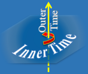
Follow inner-time generation and outer-time completion from a worked model to its physical research target.