


A fit and a prediction answer different questions
A physical proposal becomes testable when it specifies both what should be measured and what alternatives would produce different records. Reproducing a formula that was inserted into a construction is a consistency check. A distinguishing test needs an independently fixed prediction and a controlled comparison. The book makes that separation central to its research programme. [O04]
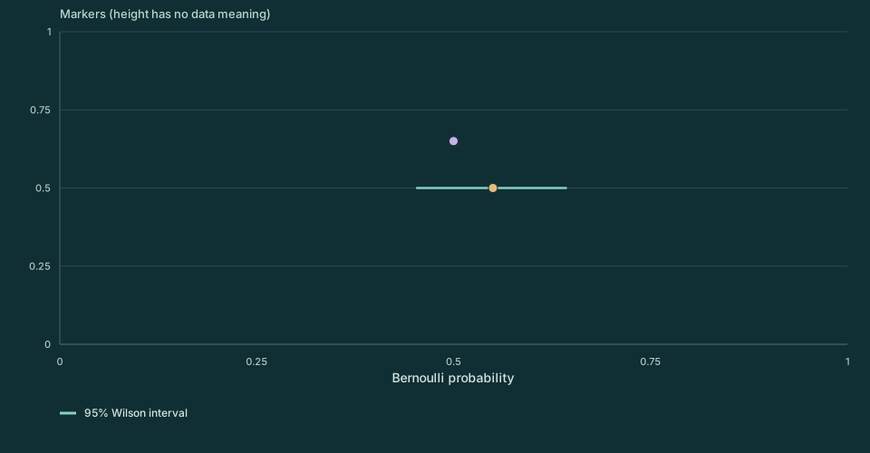
The laboratory supplies a probability p₀ and a synthetic count k out of n independent trials. It displays the observed fraction k/n and a two-sided 95% Wilson score interval. No actual experiment is connected to the page, and entering a count does not establish that its sampling assumptions hold.
The uncertainty calculation concerns a constant binary probability. It does not include detector drift, unknown efficiency, correlated trials, model selection, or repeated searching across many settings. Those effects require additional measurements or a more appropriate likelihood.
Separate disagreement from sample size
Change the number of trials n, the requested observed fraction f, and the supplied prediction p₀. The lab converts f to a valid integer count k=round(nf), then uses the actual estimate k/n. This matters for small samples: only fractions compatible with integer counts can be observed. Compare that estimate with the interval before interpreting a visible difference.
Interactive calculation
Change the inputs to compare the model outputs.
Enable JavaScript for adjustable values. The static figure and worked calculation remain available.
For the synthetic example n=400 and f=0.55, k=220 and the Wilson interval is approximately [0.5010,0.5980]. A supplied probability 0.50 lies just outside this interval; 0.54 lies inside. These are outcomes of this one fixed comparison, not a verdict on an entire physical theory. Away from probability boundaries, interval width contracts approximately as n⁻¹ᐟ².
Invert a score comparison
The formula comes from solving the score-test inequality for the unknown probability. Unlike the elementary symmetric interval p̂±z√[p̂(1−p̂)/n], it remains inside [0,1] and does not collapse to zero width merely because the observed count is zero or n. The NIST handbook gives the expression and distinguishes it from the adjusted Wald interval. [O05]
For k=0, the upper limit simplifies to z²/(n+z²), while the lower limit is zero. Thus zero observed successes does not establish a zero underlying probability. Likewise, k=n does not prove certainty.
A confidence procedure is interpreted through repeated sampling: its intervals have an intended coverage level under the assumed model. For a realized interval and fixed unknown p, it is not automatically a posterior probability statement about p. Discrete counts mean the Wilson procedure's actual coverage is approximate, not exactly 95% for every n and p.
Build a comparison that can survive repetition
Before collecting data, identify the outcomes, exposure, inclusion rule, calibrated apparatus model, parameter estimates, and reserved comparison. If p₀ was tuned to the same k, agreement is partly built into the exercise. Reserving observations or predicting a second setting makes that dependence testable.
A systematic bias does not shrink just because n grows. Independent batches, settings in a randomized order, detector reversals, and calibration checks can distinguish a model discrepancy from an apparatus effect. These are design choices for an actual study; the slider experiment supplies none of that empirical evidence.
For SMM/DTT, the next scientific step is an explicit source model whose retained-record statistics differ from a stated baseline after its scales and nuisance parameters have been fixed. The published reconstruction gives mathematical constraints that such a model must satisfy. The website's laboratories make assumptions inspectable and calculations reproducible; they do not convert a supplied standard model into a new experimental prediction. [P01] [B16]
Return to Emergence for generated records, Matter for persistent physical carriers, or the source and model register for the complete conventions used here.