
Positive response theory gives an exact capacity and a unique minimizing field. Trace normalization can produce an inverse-rank factor, while a common source dynamics must still determine stiffness, physical charge, continuum scale, action and propagation.
1. Specify the receiver, metric and physical probe
Let R be an N-dimensional complex receiver. A response variable F is Hermitian on R, so the real response space has dimension N², even though the underlying record space has dimension N. Use the Hilbert–Schmidt inner product ⟨X,Y⟩=Tr(XY). Keeping these two dimensions distinct avoids counting matrix entries as additional retained records.
Supply a positive self-adjoint linear operator K on the response space, with quadratic energy E(F)=⟨F,KF⟩/2. Positivity means every nonzero perturbation has positive cost. Supply also a nonzero Hermitian source direction f and define the imposed scalar current j=⟨f,F⟩. This equation defines the probe normalization; it cannot be changed later while claiming to preserve the same current.
The inverse K⁻¹ exists in this finite positive setting. A model with zero modes requires a separate restriction or compatibility analysis: a source overlapping a zero-cost direction can have zero minimum cost and cannot be inserted into the positive inverse formula unchanged. Here the strict assumption gives a clean theorem.
In DTT, F represents a retained response accessible at completion, while K represents its energetic resistance. Neither is the complex phase generator from the earlier chapter. The research objective is to obtain both the receiver and these response data from the same nested source process. Declaring their mathematical roles first makes that objective precise.
2. Prove the constrained minimum and its dual meaning
Minimize E(F) subject to ⟨f,F⟩=j. A Lagrange multiplier λ gives KF=λf. Defining the positive capacity Cf=⟨f,K⁻¹f⟩ yields λ=j/Cf and therefore:
For a direct proof, write any admissible F as F*+Z. The constraint gives ⟨f,Z⟩=0, so the cross term ⟨KF*,Z⟩ vanishes. The remaining energy difference is ⟨Z,KZ⟩/2, positive unless Z=0. This establishes global minimality and uniqueness without an assumption that unobserved coordinates stay fixed.
The dual experiment fixes a conjugate drive λ and minimizes E(F)−λ⟨f,F⟩ without a current constraint. Its minimizer is λK⁻¹f, its output is j=λCf, and its minimized driven energy is −λ²Cf/2. Thus Cf is an actual linear response: the derivative of output with respect to the specified drive.
A large capacity means a fixed current costs less energy, while a fixed drive produces more current. Mixing these two experimental conventions can reverse the apparent interpretation of a coefficient. In the interaction construction below, it is the fixed-flux energy that supplies the effective stiffness 1/Cf.
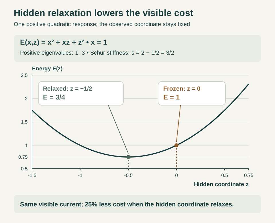
4. Calculate the 137-sector response and its bounds
Use the three record sectors of dimensions n₁=100, n₂=30 and n₃=7. If the response operator acts with positive stiffness κi on each block identity, and trace drives those identities equally, their orthogonality gives Cf=100/κ₁+30/κ₂+7/κ₃. Other directions may be supplied any positive uncoupled stiffness; they do not alter this particular probe calculation.
Equal sector stiffness κ gives Cf=137/κ. Doubling only κ₁ gives 87/κ, while leaving all 137 records available. In the fixed-current convention the energy consequently increases by 137/87. Preserving sector dimensions and each sector's internal symmetry does not force equal response weights.
Useful bounds survive without isotropy. Suppose kminI≤K≤kmaxI with kmin>0. Diagonalize K: its inverse eigenvalues lie between 1/kmax and 1/kmin. Expanding f in that eigenbasis proves:
f=IN: kmin≤s=N/Cf≤kmax
These inequalities can turn a source estimate into a controlled coupling interval even before an exact stiffness is known. If K changes smoothly, differentiating KK⁻¹=I gives δCf=−⟨K⁻¹f,(δK)K⁻¹f⟩ for a fixed probe. A positive added stiffness lowers capacity. The formula also identifies precisely which internal directions a response comparison is sensitive to.
5. Recover information with more than one source
One scalar capacity cannot identify an entire operator. Choose independently normalized probes f₁,…,fm and define the linear map A sending a vector of drive amplitudes λ to Σλafa. The response matrix is R=A†K⁻¹A. It is positive definite when the probes are linearly independent, because λ†Rλ=‖K−1/2Aλ‖².
With simultaneous imposed outputs j=A†F, minimization gives F*=K⁻¹AR⁻¹j and Emin=j†R⁻¹j/2. Multiplying the first formula by A† verifies the constraint; the same orthogonal-remainder argument proves the minimum. Off-diagonal entries measure cross-response between probes.
For K=diag(2,4), take f₁=(1,1) and f₂=(1,−1). Direct multiplication gives R=[3/4,1/4;1/4,3/4]. Its eigenvalues are one and one half. The isotropic model K′=(8/3)I agrees on each individual capacity, 3/4, but has zero cross-response. Driving one probe and reading the other distinguishes the models even after both individual capacities agree.
When the probes span the full space, the response matrix can reconstruct K⁻¹ in that known basis. Restricted probes reconstruct only their accessible part. This offers a concrete SMM/DTT research direction: derive a source-selected relation among several responses rather than assign universal significance to one fitted scalar. Relative probe orientation and normalization must be fixed independently for the comparison to carry information.
6. Derive the graph response before taking a continuum limit
Let a connected graph describe already retained spatial adjacency. Orient its edges and let B be the vertex-edge incidence matrix. Place a scalar flux je on each edge, with positive capacity Ce. The edge energy is Σje²/(2Ce). A source vector ρ obeys conservation Bj=ρ and must sum to zero on a closed finite graph.
Using a multiplier φ for conservation gives j=CedgeB†φ, where Cedge is the diagonal capacity matrix. Substitution yields Lφ=ρ with L=BCedgeB†. This weighted Laplacian annihilates constant potentials. Fixing the mean of φ, or equivalently using its inverse on the zero-sum subspace, makes the solution unique. The minimized energy is ρ†L⁺ρ/2.
This derivation explains why a Green function appears: it is the inverse of the conservation operator after internal fluxes relax. For two vertices, self-energies and the cross term follow from the same quadratic expression. With opposite unit sources the cross term is −(L⁺)uv, whose sign is not fixed for a finite graph with the mean-zero Green function. Interpreting a physical interaction requires the specified geometry and self-energy reference; record count alone does not establish attraction.
A three-dimensional inverse-distance law requires an additional controlled spatial limit. Mesh lengths, edge weights, source normalization and boundary conditions must converge to a specified continuum operator. A picture of a rank-three readout does not establish that limit. The graph calculation supplies the exact finite target whose scaling must be derived from the nested source update.
7. Match the continuum coefficient and check units
For a homogeneous three-dimensional continuum, suppose the limiting conserved-flux energy is (scont/2N)∫|J(x)|²d³x, with ∇·J=ρ. The coefficient scont already includes the graph-to-continuum scaling. For dimensionless unit source strength, J has dimensions of inverse area, so the integral has dimensions of inverse length and scont has dimensions energy times length.
Use the multiplier term ∫φ(ρ−∇·J). Minimizing gives J=−(N/scont)∇φ and −Δφ=(scont/N)ρ. Thus φ=(scont/N)(−Δ)⁻¹ρ and the minimized energy is ∫ρφ/2. Its three-dimensional Green function is 1/(4πr), established by the unit flux through a sphere and harmonicity away from the origin. The cross energy of opposite unit sources, after their separate self-energies are removed, is:
Let a be the action scale independently identified through coherent matter phase, and c the propagation speed identified by the same physical clock. The dimensionless interaction strength is g=C/(ac)=scont/(4πNac). The product ac also has units energy times length, so the primitive ratio gprim=scont/(4πac) cannot be changed by converting units.
The ideal coupling g₀=1/137 follows conditionally if N=137 and the common source proves gprim=1. Electromagnetic identification then specifies the physical charge and field convention. The factor 4π belongs to three-dimensional flux normalization; moving it between definitions must leave the final dimensionless observable unchanged.
8. Expose the calibration freedom constructively
With the probe held fixed, replacing K by λK divides capacity by λ and multiplies every fixed-current energy by λ. With K held fixed, replacing f by bf multiplies capacity by b². Neither operation changes receiver rank. The first alters stiffness; the second alters what the stated current means. A physical derivation must constrain both relative to independently identified matter variables.
Even a symmetry mixing every record could restrict K to a common isotropic coefficient while leaving its overall scale free. Such a symmetry is valuable because it removes relative sector parameters, but it does not calculate a dimensionless stiffness-to-action ratio. An argument based only on covariance must say which of these conclusions it actually proves.
One useful intermediate success is a protected ratio. If a source law fixes two capacities to C₁=a₁/κ and C₂=a₂/κ with the same unknown positive scale, then C₁/C₂=a₁/a₂ is fixed without knowing κ. A measured or separately calibrated first capacity makes the second a conditional prediction only if the probe definitions and the shared-scale law were fixed beforehand.
For the full coupling problem, freeze the architecture, response operator, source normalization and action–clock dictionary before using atomic data. Calculate the allowed values across all models still satisfying those inputs. A unique value, or a controlled interval with a reason why rescaled countermodels are excluded, is a noncircular result. Reproducing a number used to choose κ establishes calibration consistency instead.
9. Connect the achieved response to the source programme
The positive theorem is substantial: a declared response model has a unique minimizing field, a measurable capacity, an exact hidden-mode reduction, computable bounds and a multi-probe reconstruction rule. Conservation converts edge capacities into a graph Green function. With a justified three-dimensional limit, this yields a Coulomb coefficient with explicit units.
SMM/DTT can use these statements to formulate a sharper common-source challenge. The six inner roles must build the same retained receiver whose response also defines matter propagation, while the seventh completion interface reports the currents, positions and clock readings used in matching. These roles are nested dependencies, not six independent clocks to be tuned separately.
The required new law should constrain a joint output, such as scont/(ac), rather than merely prescribe another label for 137. A finite solvable source could first establish an invariant multi-probe ratio or a stiffness bound. A stronger model could derive the normalized coupling itself. Both are clear advances when their assumptions and remaining freedom are stated.
The hydrogen chapter now inserts the supplied C into one atomic Hamiltonian. Radius, energy and relative momentum then follow together. Their agreement tests the response-to-matter dictionary; it does not retrospectively select the coupling from the existence of binding. The response workbench keeps count and stiffness controls distinct so this dependence remains visible.
Continue with the articles
- Why a record count is not yet a coupling
A receiver's static response depends on its source and inverse stiffness, as well as its size. Exact minimization shows why counting 137 records does not by itself determine an electromagnetic coupling.
- Trace-sector response and the Schur complement
Allowing hidden traceless modes to relax changes the stiffness seen by a trace source. The Schur complement gives the exact reduced capacity and exposes the normalization still needed for an inverse-rank coupling.
- The conditional ideal value one over 137
The ideal model value 1/137 requires a selected record count, a trace-response law, and an additional absolute normalization. A hydrogen-like calculation checks their consistency without deriving the measured fine-structure constant.
- Why normalized response misses absolute vacuum offsets
Normalized responses erase source-independent offsets even when those offsets matter to an absolute functional. The exact obstruction explains why stiffnesses, spectral ratios, and temporal averaging do not alone determine gravitating vacuum energy.
- An exact singlet-loop response
A mobile carrier, stationary dual, and supplied singlet-binding Hamiltonian reduce to one exact resolvent equation. Its unique physical root determines the holonomy-dependent ground response and a conditional completion-cost candidate.
- A normalizable hydrogen-like ground state
Square completion gives the exact normalized ground state of the supplied nonrelativistic Coulomb Hamiltonian. Its spectrum and relative root-mean-square speed provide precise atomic benchmarks without selecting the coupling itself.
- Why binding does not fix the coupling
Dilation shows that every positive Coulomb coupling admits binding and the same type of ground-state filter. A source derivation of a particular coupling must therefore fix field, matter, action and clock normalization beyond the existence of an atom.