
A prediction becomes informative when fixed assumptions and independently calibrated parameters restrict a new observable across every remaining admissible model.
What you will learn
- Separate proved statements, supplied inputs and physical interpretations.
- Test whether calibration leaves a target observable undetermined.
- Design an overconstrained comparison with fixed parameters and explicit alternatives.
Before you begin: Lessons 01–11. This final lesson uses the record, geometry, phase, clock, gauge, matter and response distinctions developed throughout the course.
Attach a claim to its actual premises
For each result, write its input, calculation and output. The binary counter begins with a signed paired readout and yields 27 sites. Polar phase selection begins with an oriented invertible skew generator and yields J²=−I. The Coulomb calculation begins with a Hamiltonian and yields a bound state. These are positive exact results, each with a different dependency.
Next identify the proposed physical interpretation. Calling the sites space, the phase a material clock or the bound state hydrogen requires operational matching. The research claim map and model-consistency guide organize these checks. A missing interface does not erase an earlier theorem; it tells us which additional construction would extend its explanatory reach.
Worked example: one calibration leaves freedom
Suppose a model has parameters a and b. A calibration fixes a+b=3, while the target output is Y=a−b. Two allowed choices, (a,b)=(2,1) and (1,2), satisfy the same calibration but give Y=1 and Y=−1. Therefore the calibration alone does not predict Y.
The set of parameter choices satisfying the calibration is the remaining calibrated family. A target is fixed only when it has the same value across that whole family, within declared errors. A source law imposing b=a/2 would reduce the example to a=2,b=1 and predict Y=1. But fitting b=a/2 after measuring Y=1 would reuse the target. The order in which information enters matters to the evidential claim.
Use an alternative that obeys the same early results
Consider a refinement construction with record dimension D and an inner quantity u=Dτ. A proposed clock reads T=τ, giving u/T=D. An alternative clock can read T=τ+λu while preserving the same record count and inner relation. Then u/T=D/(1+λD).
For D=2 and D=3, λ=0 gives two and three, whereas λ=1 gives 2/3 and 3/4. No single fixed rescaling makes the two clock laws agree across both settings. This countermodel identifies a meaningful selection question: what source interaction excludes or fixes λ? Merely naming one device the outer clock cannot establish universal clock response. A useful theorem constrains the competing interaction through independently justified source dynamics.
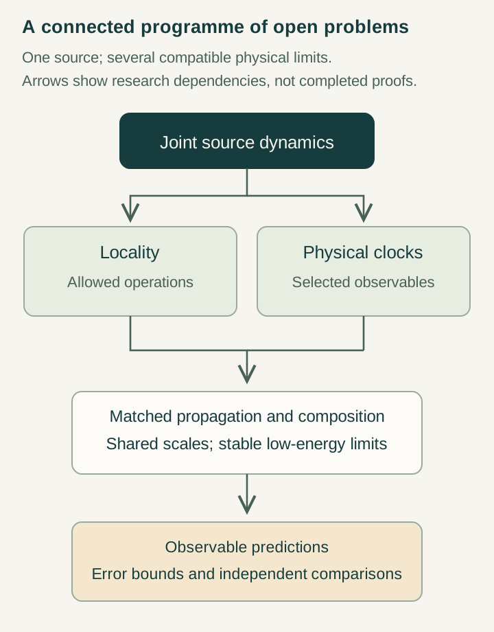
Open the full-size diagram →
Use the demonstrations as six separate checks
The nested-generation demo tests dependency and address counts. The binary readout tests multiplicity and lost carry memory. The phase rotation tests the quarter-turn algebra. The clock comparison tests a supplied relativistic benchmark.
The gauge loop tests endpoint cancellation, while the binding curve tests the supplied Coulomb energy family. Reproducing each default is a consistency check. The common-source challenge is to derive a shared restriction connecting their inputs, so one calibrated output fixes another. Six individually correct demonstrations do not automatically form one autonomous physical model with a shared memory, clock and action scale.
Read published results at their own level
The published completion framework organizes observable quotients, compatible phase structures and conditional cone readouts. The real-commutant paper treats phase selection for real Hilbert representations. The temporal-asymmetry paper uses coupled temporal coordinates and projected memory descriptions. Their paper guides help locate assumptions and follow the original sources.
The later nested-counter constructions are not automatically identical to the published two-coordinate formulation. An explicit translation must identify state spaces, operations, observables and completion. Nor do the three papers by themselves establish every receiver grammar, gauge group, Pauli law, Einstein equation or Yang–Mills gap discussed elsewhere in the programme. Evaluate each claimed bridge through the particular result and hypotheses that support it.
Design a comparison that can change your conclusion
Choose an accessible target and an alternative model before looking at the target result. Calibrate only the allowed parameters, freeze them, then predict several settings with the same values. Include failed or incomplete outcomes, apparatus uncertainty and memory preparation. A residual is interpretable only after ordinary responses covered by the comparison model are accounted for.
For an atomic example, use one coupling and reduced-mass dictionary to predict radius, binding energy and momentum relations together, then declare which corrections are included. For a memory example, fit one response protocol and predict another without changing the kernel. The prediction guide develops this workflow. The course's final question is concrete: which new relation does the common source enforce that its explicit alternatives do not?
Try the exercises
Work through each question, then open the answer to compare the steps.
Exercise 1
A calibration fixes ab=6 for positive parameters. The target is a+b. Compare (a,b)=(2,3) and (1,6). Has the target been predicted?
Show the worked answer
Both pairs satisfy ab=6. Their target values are 2+3=5 and 1+6=7, so the calibrated family leaves the target undetermined. A further independently justified relation, such as a=b, would give a=b=√6 and target 2√6. Imposing that relation because it fits the already observed target would not be an independent prediction.
Exercise 2
A source model is fitted to one hydrogen radius and then reports that same radius as a success. It also gives a ground binding energy from the fixed parameters. Classify the two outputs and state a fair next check.
Show the worked answer
The fitted radius is a calibration output, so reproducing it checks implementation but supplies no independent predictive success. The binding energy is a conditional prediction if every coefficient and correction entering it was fixed without using that energy. A fair next check compares the frozen energy prediction with its independent target and stated uncertainty, then tests another transition or isotope using the same interaction law and separately supplied mass inputs.
Continue with the articles
- Prediction after calibration
Calibration produces a prediction only when the proposed output is fixed across the remaining admissible models, or constrained to a stated range. This criterion distinguishes cross-sector consequences from reuse of a fitted target.
- Why one clock model does not prove universality
Protected and ungated clocks can coexist with the same record geometry while assigning different readings to it. This countermodel shows why constructing one desired clock does not establish a universal material-clock law.
- Six inner stages and one publication interface
A six-digit nested counter with paired signed readout realizes ranks 1, 1, 2, 2, 3, 3 before one completion interface. Its exact counts reveal sampling bias and the restricted assumptions behind the six-channel bound.
- Freeze parameters before predicting spectroscopy
A spectroscopy test becomes predictive when its operator family, coefficients and calibration data are fixed before the reserved transitions are examined. The freeze record makes the dependency between constants and atomic predictions auditable.
- Designing an overconstrained atomic test
An overconstrained atomic test compares independent residual directions with a declared set of source and nuisance coefficients. Covariance weighting and singular-value analysis reveal whether the chosen observables can actually distinguish the proposed mechanism.
- Real-commutant phase selection: a paper guide
An oriented real orthogonal flow can select an ordinary complex structure on its dynamic sector. Planar examples explain residual zero-mode freedom, time-reversal antilinearity and the extra balancing rule needed for composite systems.
- Temporal asymmetry: reading the published model
The temporal-asymmetry model connects projected dynamics with memory and path dependence. A solvable hidden-mode example distinguishes those effects from dissipative stability and from evidence for a second observable clock.