


Assumptions, results and research status
Leading Dirac–Coulomb benchmark; temporal operator descent remains open
Assumptions
- The explicit operator derivation uses an electron of mass mₑ and a point nucleus of infinite mass, with no external fields.
- The expansion retains energy corrections through order α⁴ and omits radiative and nuclear effects.
- The electron has the usual spin-one-half representation and the minimally coupled Dirac benchmark is supplied.
Results
- Relativistic kinetic, spin–orbit, and Darwin terms combine into one n,j-dependent correction.
- The leading 2P₃/₂–2P₁/₂ interval is mₑc²α⁴/(32h).
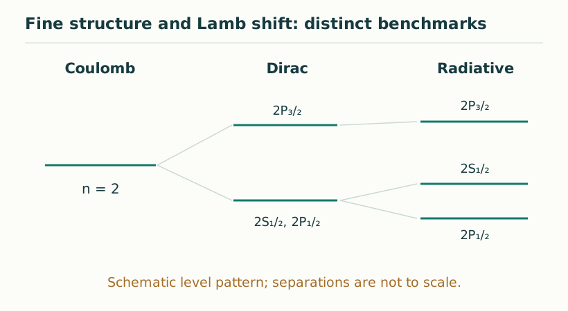
- The point-Coulomb Dirac model leaves 2S₁/₂ and 2P₁/₂ degenerate; their Lamb interval requires additional physics.
Open question: Can the temporal source construction fix the effective spinor dynamics and all three fine-structure coefficients without independently imposing the Dirac–Coulomb operator?
1. Resolve the spectrum one physical layer at a time
The gross Coulomb binding energy is of order mec²α². Typical atomic momentum is of order mecα, so relativistic corrections to that motion naturally begin two additional powers of α below the gross scale. This scale estimate explains why fine structure is small, but it does not determine the signs, coefficients, or state dependence of the splitting.
Those details require an operator calculation. A convenient benchmark is a spin-one-half electron in the electric field of a fixed point proton. The infinite-nuclear-mass assumption is deliberate here: it makes the relativistic derivation unambiguous. Reduced mass and higher recoil effects can be restored through a consistent two-body treatment.
Paper 13 organizes the kinetic, spin–orbit, and Darwin contributions and identifies descent from temporal records to the effective Dirac description as an additional theorem target. [Paper 13, §§4 and 23] The aim of this article is to make the resulting numerical benchmark explicit enough that a proposed source construction can be checked term by term.
Throughout the calculation below, write m = me, k = αℏc, and V(r) = −k/r. Energies are internal binding energies, with the electron rest energy subtracted.
2. The relativistic kinetic correction
Expand the relativistic free-particle energy in powers of p/(mc):
The first term belongs to the Coulomb Hamiltonian. The next term supplies Hkin = −p⁴/(8m³c²), a negative first-order correction. It is an effective low-momentum expansion, not a replacement Hamiltonian to be extrapolated to arbitrarily large p, where the truncated polynomial would become unbounded below.
For a Coulomb eigenstate, p²ψ = 2m(E − V)ψ. This identity converts the p⁴ expectation into radial moments of V and V². Using ⟨1/r⟩ = 1/(a0n²) and ⟨1/r²⟩ = 1/[a0²n³(ℓ + 1/2)] gives
This term depends on ℓ, not only on n. It therefore breaks some of the scalar Coulomb degeneracy. It also shows why a characteristic-speed substitution alone cannot recover the full answer: different angular states at the same principal number have different higher momentum moments.
3. Spin–orbit coupling fixes an angular pattern
The leading spin–orbit term in the same benchmark is
The factor 1/2 is part of the relativistically consistent coefficient. It cannot be chosen independently after comparing the splitting. The angular dependence becomes transparent in states of J = L + S, with electron spin s = 1/2:
For ℓ ≥ 1, the possible j values are ℓ − 1/2 and ℓ + 1/2. The spin–orbit eigenvalue is negative for the first and positive for the second. Its radial factor involves ⟨1/r³⟩ = 1/[a0³n³ℓ(ℓ + 1/2)(ℓ + 1)], valid for ℓ ≠ 0.
The apparent singularity of that radial formula at ℓ = 0 does not justify inserting an arbitrary value. S states have zero orbital angular momentum, and their short-distance relativistic contribution is handled by the separate Darwin term. This is one reason the operator formulation is safer than a classical orbit picture of spin precession.
4. The Darwin term completes the S-state result
The Darwin contribution in the point-Coulomb benchmark is
The distributional identity ∇²(1/r) = −4πδ³(r) fixes its sign. Since V = −k/r, the contact coefficient is positive. At first order, only S states contribute because their Coulomb wavefunctions are nonzero at the origin:
The three-dimensional delta is used as an effective perturbative insertion with a specified origin. It is not introduced here as an unregulated standalone potential with an arbitrary bound-state spectrum. The same mathematical caution applies to later contact models for nuclear size or a proposed temporal correction.
The kinetic, spin–orbit, and Darwin pieces depend on the representation used for the effective theory. Their combined level shifts are the physical benchmark. An interpretation that associates each piece with temporal motion, orientation, or completion still needs a derivation of their shared normalization and relative coefficients.
5. The combined n,j formula and the Dirac check
Adding the three first-order contributions cancels the separate ℓ dependence in the required way. The result is
The dependence is on n and j. It is the order-α⁴ term in the exact point-Coulomb Dirac spectrum. One way to check the expansion is to define D = n − j − 1/2 + √[(j + 1/2)² − α²], then expand
Subtract mc² before comparing with binding energies. The expansion first produces −mc²α²/(2n²), then the displayed fine-structure correction. This agreement checks both the coefficient and the angular pattern. MIT’s fine-structure notes provide an independent presentation of the standard calculation. [MIT, Hydrogen Fine Structure]
The remaining degeneracy is also a prediction. States with the same n and j but different allowed ℓ remain degenerate in this ideal Dirac–Coulomb problem. In particular, 2S1/2 and 2P1/2 still coincide. A theory should reproduce that intermediate benchmark before explaining how radiative and other corrections lift it.
6. Worked example: resolve the n = 2 multiplet
At n = 2, direct substitution gives the following shifts, measured relative to the common nonrelativistic n = 2 energy.
| State | j | δEfs/(mc²α⁴) |
|---|---|---|
| 2S1/2 | 1/2 | −5/128 |
| 2P1/2 | 1/2 | −5/128 |
| 2P3/2 | 3/2 | −1/128 |
Using the declared reference constants gives approximately 10.9493 GHz for this leading infinite-mass formula. This is a computed approximation, not a quoted precision measurement of physical hydrogen. Replacing m by μ in the compact expression gives about 10.9433 GHz, but that replacement alone is not the complete two-body recoil correction. [NIST CODATA inputs]
The interval has four powers of α when m and h are held fixed, so a small change in α gives a leading fractional change 4δα/α. That sensitivity is conditional on the chosen independent inputs; it does not supply a derivation of α.
7. Restore recoil, radiation, and nuclear structure consistently
The proton moves. At the gross level this motion is handled exactly by separating the nonrelativistic two-body problem and using reduced mass. At relativistic order, additional two-body kinetic and interaction terms appear. A consistent recoil treatment derives these terms together instead of substituting μ into every electron-mass denominator.
Radiative corrections modify the point-particle benchmark further. Nuclear charge distribution, magnetic structure, and hyperfine interactions introduce additional state dependence. External electric and magnetic fields can mix or split levels, changing which labels remain exact. The CODATA hydrogen and deuterium review treats these contributions in a coordinated bound-state calculation. [CODATA review, §III]
Each comparison should state whether it concerns an individual hyperfine component, a centre of gravity, or an unresolved line. Theoretical and tabulated quantities must represent the same object. A number obtained by averaging over several components cannot be compared directly with one selected component simply because their principal n values agree.
The Lamb-shift article develops the radiative layer; hyperfine structure and isotopes explains the separate role of nuclear spin and mass.
8. A precise target for temporal spin and propagation
A temporal spin interpretation can motivate why a spinorial description might occur. A complete hydrogen result must additionally derive the effective spinor operator, its coupling to the Coulomb field, and the normalization that produces the kinetic, spin–orbit, and contact terms above. A 4π return property alone does not determine those coefficients.
Paper 13 makes the effective Dirac descent and radiative coefficient calculations explicit targets. [Paper 13, theorem and coefficient ledgers] A productive first theorem would obtain the order-α⁴ operator from one regulated source model and show that it reduces to the displayed combination under the stated limit.
Such a result should include a controlled error estimate and identify which source symmetries protect the angular pattern. It should then use the same coefficients for all n and j, including the surviving 2S1/2–2P1/2 degeneracy at this stage. That combination of a nonzero splitting and a protected degeneracy is a demanding, concrete test of the proposed temporal account.
Continue reading
Sources for this guide
Source manuscripts, version notes, and standard references are listed in the reference library.