


Assumptions, results and research status
Exact linked scale relations in the Coulomb model; structural selection and physical electromagnetic matching remain distinct tasks.
Assumptions
- The same constants and reduced mass are used in the kinetic, interaction, and clock normalizations.
- The velocity statistic is the quantum relative RMS speed, with the finite-mass correction stated for the electron.
- The value 1/137 is used only as an explicitly illustrative structural-coupling hypothesis, not as the measured electromagnetic coupling.
Results
- The leading scales satisfy a = ħ/(μcg), B = μc²g²/2, and Ba = għc/2.
- The relative RMS speed is cg/n; the electron RMS speed in the centre-of-mass frame is smaller by μ/mₑ.
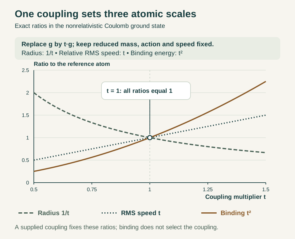
- Changing a proposed coupling produces correlated radius, energy, and frequency shifts that cannot be adjusted independently.
Open question: Can a temporal response law fix the physical coupling from structural completion data and independently calculated corrections, with the same normalization governing hydrogen?
Define the coupling through an operator
Write the effective interaction as −C/r and define g = C/(ħc). This dimensionless number compares the attractive response with the action and speed scales used in matter propagation. Electromagnetic matching identifies g with alpha only after those conventions and the physical response have been specified.
μ = memp/(me+mp)
The distinction is useful because the mathematical Coulomb problem exists for every g > 0. Its bound states do not select one special coupling. A source theory must constrain C relative to the same ħ and c used elsewhere, rather than infer the coupling from the existence of a normalizable atom.
Paper 12 keeps the constants as independently supplied inputs to its effective reconstruction. The later hydrogen calculation then reveals their consequences without allowing the spectrum to choose the inputs again. [Paper 12, §§2–4]
Reduce the leading atom to one universal shape
Define a = ħ/(μcg) and B = μc2g2/2. Rescale position by x = r/a and the wavefunction by a−3/2 so normalization is preserved. The Hamiltonian becomes:
En/B = −1/n2
All positive couplings share this dimensionless leading Coulomb shape. Their physical radii and energies differ because a and B differ. This explains why matching a scale-free pattern such as the leading ratios of spectral intervals does not by itself determine the physical coupling.
The finite proton mass enters through μ. Compared with the conventional Bohr radius a0 defined using me, the relative radius is aμ = a0(1 + me/mp). The leading energy scale is reduced by μ/me. Both effects follow from one two-body separation, not separate atomic adjustments.
The linked scales explorer makes these dependencies visible while keeping its approximation and input values explicit.
State exactly what alpha equals in the ground state
In the effective relative-coordinate model, the velocity operator is vrel = p/μ. The normalized ground state gives ⟨p2⟩ = ħ2/a2, so its root-mean-square relative speed is cg. The virial relation extends the result to the bound Coulomb energy levels:
ve,rms/c = (μ/me)g/n in the centre-of-mass frame
After matching g = α, the ground-state relation is vrel,rms/c = α. The electron’s corresponding centre-of-mass quantity includes the finite-proton-mass factor. Taking an infinitely heavy proton makes that factor approach one.
A real scalar ground-state wavefunction has current j = (ħ/μ)Im(ψ*∇ψ) = 0. Its positive RMS speed is a momentum statistic, not a steady flow around a classical orbit. The existing RMS-speed derivation makes this distinction explicit.
The canonical-complexification draft also discusses a circular effective approximation and its finite-mass dictionary. The quantum statistic above gives the sharper statement for the actual scalar ground state. [Canonical-complexification draft, §16]
Use the linked sensitivities as consistency checks
Hold μ, ħ, and c fixed and change g by a small fraction. The radius changes by the negative of that fraction, while the binding magnitude and leading spectral frequencies change by twice that fraction:
δB/B ≈ 2δg/g
δν/ν ≈ 2δg/g
If the masses or unit dictionary also change, their contributions must be included. For example, a depends on μ−1 and B on μ, so a reduced-mass change affects the two scales with opposite signs. The exact relations provide useful cross-checks:
Ba2 = ħ2/(2μ)
The second identity eliminates the coupling entirely. Recovering radius and energy together is therefore more informative than matching either one with an adjustable normalization.
These relations are exact within the leading model and their linearized versions apply to small parameter changes. A new interaction need not act as a uniform change of g: its state-dependent expectation values can produce a different pattern. Such a proposal should be written as an operator and compared through its shared level shifts.
Keep structural completion counts and couplings connected precisely
The proposed structural expression
is an exact arithmetic result for its supplied multiplicities and weights. Its role in SMM/DTT is to be assessed through the construction that selects those ingredients. The canonical-complexification draft separates this structural integer from a physical electromagnetic coupling and identifies further response and correction work. [Canonical-complexification draft, §§14–16]
Where 137 and 128 describe different structural completion sectors, their comparison belongs first to those sector definitions. They should not be assigned low- and high-energy electromagnetic meanings without an independently derived physical scale dependence.
A candidate relation g = 1/(137 + Δ) is predictive only when Δ and the normalization connecting the count to g are fixed without using the same hydrogen observations reserved for assessment. Writing a measured discrepancy into Δ reproduces a number, but it does not establish the physical mechanism responsible for it.
Worked example: an ideal 137 hypothesis
As a transparent illustration, suppose gtoy = 1/137 while the other inputs are held fixed. The 2022 CODATA reference table gives α−1 = 137.035999177, with standard uncertainty 0.000000021. This supplies an identified comparison value rather than an unnamed approximation. [NIST 2022 CODATA]
atoy/aref = 137/137.035999177 ≈ 0.99973730
Btoy/Bref ≈ 1.00052560
The illustrative coupling is about 0.0263% larger, the characteristic radius about 0.0263% smaller, and the leading binding magnitude about 0.0526% larger. The same fractional binding change applies to all leading Coulomb intervals when only this coupling is changed.
This is a sensitivity calculation, not a claimed new spectroscopic effect. The physical interpretation would require an independently computed response correction and a consistent treatment of the additional terms needed for precise hydrogen theory. It demonstrates why the fractional part after 137 matters once a structural proposal is connected to an observable coupling.
Define temporal scales without a reciprocal ambiguity
A recurrence scale defined from the electron rest energy is τC = ħ/(mec2). If one then defines τg = gτC, its reciprocal frequency is mec2/(għ), not gmec2/ħ. The two expressions differ by a factor g2.
Such definitions can organize scales but do not derive g if g was used to construct the time in the first place. The newer hydrogen sequence treats the electromagnetic recurrence scale as downstream of the coupling input. [Paper 12]
A separate illustrative hop model could posit one distance ℓ per tick τ for a reference signal and the same distance per N ticks for another process. It then gives c = ℓ/τ and v = c/N. To compare that result with hydrogen, a theorem must connect this operational motion statistic to the quantum relative RMS observable derived above.
The common distance, tick, and physical interpretation of N are therefore substantive inputs. Identifying N with a structural count does not by itself establish the required quantum correspondence.
What an independent prediction would look like
A clear calculation record should identify the source construction, its regulator, the rule selecting the relevant sector, the independently fixed physical constants, and the approximation used for the atom. It should then compute the energy, radius, momentum statistic, and spectral intervals without changing those choices.
Reference constants and proposed source outputs serve different roles in this process. Reference inputs allow a reliable demonstration of the effective model. A source prediction requires the declared upstream derivation and an account of which measurements, if any, were used for calibration. Paper 12 emphasizes this ordering to prevent the spectrum from selecting its own inputs. [Paper 12]
Precision comparisons additionally require uncertainty and covariance information. Several reported constants and atomic quantities may share calibration data, so agreement between them need not represent independent tests.
The strongest next result would be a response law that fixes the physical coupling and then yields these linked hydrogen consequences with one common normalization. The research-status page and collaboration projects identify the remaining mathematical work needed for that step.
Continue reading
Sources for this guide
Source manuscripts, version notes, and standard references are listed in the reference library.