


Assumptions, results and research status
Coulomb benchmark with an explicit SMM/DTT derivation target
Assumptions
- A nonrelativistic electron and point proton interact through the supplied Coulomb potential.
- The relative wavefunction belongs to the usual three-dimensional square-integrable state space.
- The electromagnetic coupling, action scale, masses, and clock conversion are declared inputs.
Results
- The bound energies are Eₙ = −B/n², with B = μc²α²/2 and a zero ionization threshold.
- One common energy ladder fixes every gross interval and its series limit.
- Dimensionless ratios test the spectral form separately from the absolute frequency scale.
Open question: Can one independently specified temporal proton–electron construction generate the Coulomb operator, its normalization, and the operational energy-to-frequency correspondence together?
1. Choose the energy zero and the physical model
Place the energy zero at an electron and proton infinitely far apart, with no relative kinetic energy. A negative energy then describes binding: energy must be supplied to reach the separated-particle threshold. The rest energies of the particles are omitted from this internal Hamiltonian because they cancel in an ordinary transition between states of the same atom.
Let r be the proton–electron separation and let μ = memp/(me + mp) be the reduced mass. Separating free centre-of-mass motion leaves the internal problem
The kinetic term describes relative motion. The attractive potential is an input to this benchmark. Paper 12 derives the standard bound spectrum after this effective Hamiltonian and the physical constants have been supplied; obtaining that Hamiltonian from the temporal construction is a separate central target. [Paper 12, §§2–5]
This separation is useful for an SMM/DTT account. A temporal interpretation of the wavefunction can be developed alongside the calculation, while the calculation itself states exactly which operator and boundary conditions determine the numbers.
2. Why only certain negative energies are allowed
For a central potential, write ψ(r,θ,φ) = R(r)Yℓm(θ,φ) and set u(r) = rR(r). The radial equation contains a centrifugal term ℏ²ℓ(ℓ + 1)/(2μr²). For a bound energy, define the positive inverse length κ = √(−2μE)/ℏ. The large-distance solution must decay like exp(−κr), while regularity at the origin selects the behaviour rℓ+1 for u.
Extracting those factors leaves a power series. Normalizability requires its growing branch to terminate. If the remaining polynomial has nonnegative degree nr, termination imposes
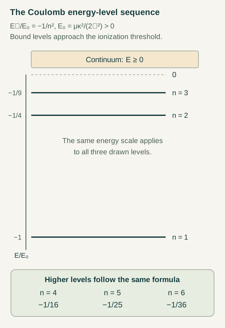
Substituting κ back into the energy gives En = −μc²α²/(2n²), where n = 1, 2, 3, …. This is a consequence of the differential equation and its boundary conditions. It is stronger than assigning the desired 1/n² values to an otherwise unspecified diagonal operator, because the same equation also determines the spatial eigenfunctions and their angular structure.
The complete solution includes a positive-energy continuum as well as the discrete negative levels. The bound levels accumulate at zero; the accumulation is the approach to ionization, not a sequence of ever more deeply bound states.
3. Quantum numbers identify states, not separate temporal axes
The principal number n determines the gross energy. For each n, the orbital number satisfies ℓ = 0, …, n − 1, and the magnetic number satisfies m = −ℓ, …, ℓ. The letters S, P, D, and F denote ℓ = 0, 1, 2, and 3. These are labels of angular-momentum representations and radial solutions.
At n = 2 there is one 2S spatial state and three 2P spatial states, all with the same energy in this scalar Coulomb approximation. Electron spin doubles the state count before spin-dependent interactions are included. Proton spin supplies further labels when hyperfine structure is resolved. MIT’s hydrogen notes provide a conventional reference for this separation and degeneracy. [MIT, Hydrogen Atom II]
The six nested inner generative levels in SMM/DTT have a different role: they concern the proposed construction of spatial and physical records. Connecting them to n, ℓ, m, and spin requires a map from source states to these representations. A visual resemblance or a matching count alone does not supply that map. The question becomes mathematically productive when the source construction fixes allowed sectors, their multiplicities, and the action of rotations.
4. A worked reduced-mass energy ladder
Define the positive binding scale B = μc²α²/2. With the 2022 CODATA input values used for the reference calculation, B is approximately 13.59829 eV for the reduced-mass Coulomb model of ordinary hydrogen. The infinite-proton-mass value is approximately 13.60569 eV. These are calculated model values; the reduced-mass result still omits relativistic, radiative, and nuclear corrections. [NIST CODATA inputs]
| n | En/B | Approximate En | Energy needed to ionize |
|---|---|---|---|
| 1 | −1 | −13.59829 eV | B |
| 2 | −1/4 | −3.39957 eV | B/4 |
| 3 | −1/9 | −1.51092 eV | B/9 |
| 4 | −1/16 | −0.84989 eV | B/16 |
The 1 → 2 energy interval is 3B/4, approximately 10.19872 eV. Dividing by h gives approximately 2.46604 × 10¹⁵ Hz. Taking c/ν gives a vacuum equivalent wavelength of about 121.568 nm. The frequency is the full level separation; a particular excitation process may distribute that energy between more than one photon.
Displayed digits should match the approximation. Additional calculator digits measure numerical evaluation of the formula, not an improvement in the physical accuracy of that formula.
5. Lyman, Balmer, Paschen, and their limits
For an upper principal number nu and a lower number nl, the positive gross frequency is B(1/nl² − 1/nu²)/h. The corresponding vacuum wavenumber is
Fixing nl creates a series. The Lyman series ends at nl = 1, Balmer at 2, and Paschen at 3. Sending nu to infinity gives the series limit λlimit = hc nl²/B. The high members crowd together because successive energy gaps shrink.
For the Balmer 3 → 2 interval, the present model gives about 1.88865 eV and 656.470 nm in vacuum. A familiar wavelength near 656.3 nm is often quoted in air. Air and vacuum conventions, fine-structure components, and unresolved blends must be aligned before numbers are compared. NIST’s hydrogen tables explicitly distinguish these cases. [NIST hydrogen lines]
6. An energy difference does not determine a line’s intensity
The energy spectrum identifies possible energy changes. It does not, by itself, determine which changes couple efficiently to a radiation field. A transition calculation additionally needs a coupling operator, state wavefunctions, and the radiation or preparation conditions. In the electric-dipole approximation, the relevant matrix element is a component of ⟨b|er|a⟩.
Consequently, 2P → 1S is an allowed one-photon electric-dipole channel, whereas 2S → 1S has a vanishing electric-dipole matrix element in the unperturbed atom. The latter can proceed through a two-photon channel. Both share the same leading principal-level separation, but they have very different transition mechanisms. The selection-rules article develops the angular and radial calculation.
Absorption and emission also depend on state populations. A hot discharge and a beam prepared almost entirely in the ground state need not show the same line pattern, even when their atoms have the same underlying Hamiltonian. Widths and line profiles require lifetimes, field effects, motion, and instrumental response. An energy-level explorer therefore displays energy intervals and declares any additional transition rules it applies.
7. Separate the spectral shape from the clock scale
Ratios remove the common binding scale. For example, the 2 → 3 interval is 5B/36, so its ratio to the 1 → 2 interval is exactly 5/27 in this model. That is a check of the 1/n² structure. It cannot separately determine μ, α, c, or h, because their common contribution has cancelled.
The second identity uses signed frequencies, νa→b = (Eb − Ea)/h. It follows from one consistent set of levels and remains true when compatible corrections are added. Positive emission-frequency magnitudes need their directions recorded before this identity is applied.
In a stationary superposition, the relative phase evolves at angular frequency (Eb − Ea)/ℏ. The ordinary cycle frequency is smaller by 2π. This phase-to-clock relation is particularly important for DTT: a count of generative cycles must be connected to an independently defined outer-time reading before it becomes a frequency in hertz.
8. What a temporal derivation should deliver
The complete target is a linked construction of the state space, effective operator, normalization, and observable clock. A source model should explain why its long-distance states have the required three-dimensional radial behaviour, why the interaction is attractive and proportional to 1/r over the stated regime, and why its strength is the same coupling obtained in the independent electromagnetic response calculation.
It should then recover normalizable eigenstates and their degeneracies, followed by transition operators and corrections. Paper 21 organizes these requirements as a dependency chain connecting the temporal construction to atomic observables. Its synthesis provides a research programme rather than an already completed physical coefficient calculation. [Paper 21, §§4–8 and Appendix F]
A useful intermediate result would reproduce the radial operator and its spectrum in a controlled limit of a finite source model, with an error bound that improves as the regulator is refined. A stronger result would fix the energy and clock scales from the same independently specified dynamics. These are concrete places where mathematical and theoretical-physics collaboration can turn the hydrogen example into a more restrictive account of atomic structure.
Continue reading
Sources for this guide
Source manuscripts, version notes, and standard references are listed in the reference library.