Refinement, dimension and the clock comparison

Measure growth before naming a dimension

Imagine repeatedly resolving each completed record into finer distinguishable children. Let B be the number of children and let q>1 be the factor by which the comparison scale improves. Count children using the declared tests and measure scale using an independent comparison procedure. Neither reading should be defined from the other.

This is a natural SMM/DTT setting: inner work produces more resolved distinctions, while outer completion makes a new level of the archive available. The six nested inner roles can organize that work without themselves being six dimensions. Dimension is inferred from the output's scaling, rather than by counting the names of its generative stages.

The exact uniform refinement law

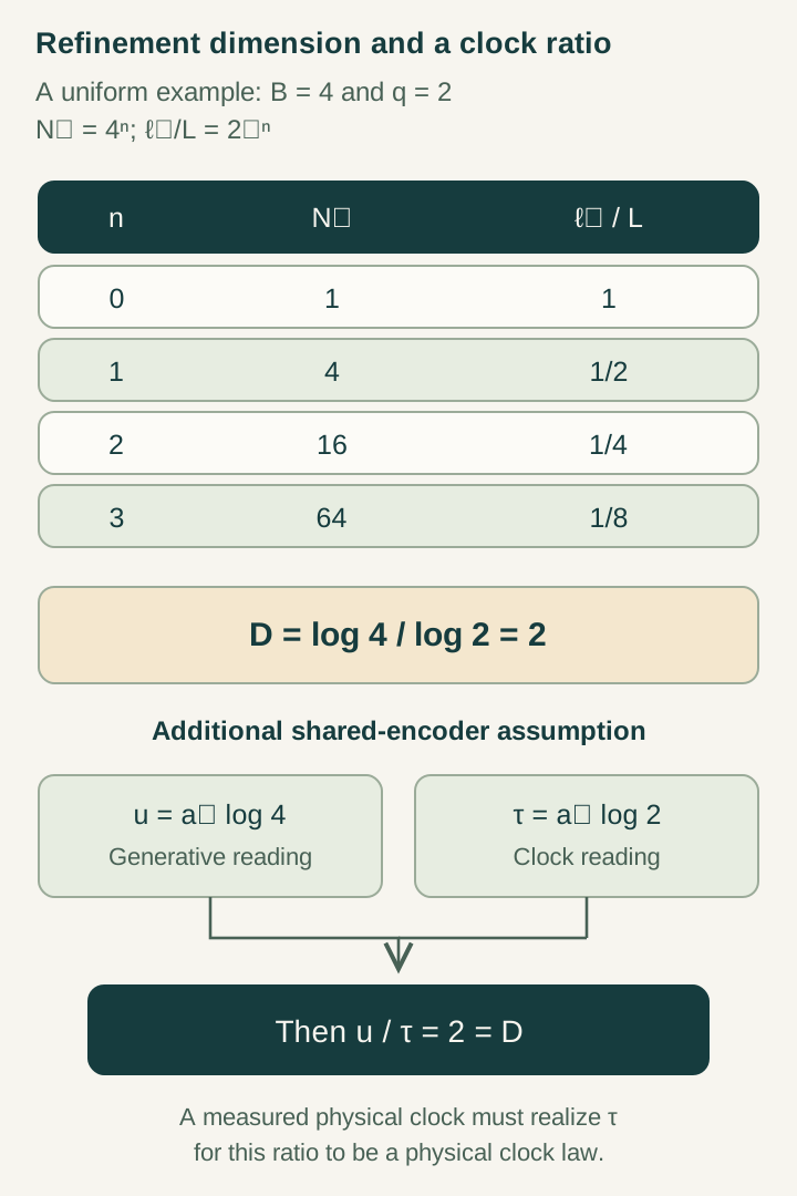
After n levels there are Bⁿ records and the comparison length is Lq⁻ⁿ. Eliminating n gives a power law between count and scale:

For an infinite address space equipped with the usual common-prefix ultrametric, level-n cylinders have diameter proportional to ℓ_n and equal probability B⁻ⁿ. Their mass therefore scales as diameter to the power D. The matching cover and mass bounds establish dimension D for this specified geometry. A finite archive alone has no nontrivial limiting dimension without a declared refinement family.

Worked example: eight children and halved scale

Choose B=8 and q=2. Four refinement levels give 8⁴=4096 distinguishable cells at scale L/16. The exponent is three because 4096=16³. The same result holds at every depth:

Keeping q=2 while changing B gives a useful family. B=4 yields D=2, and B=6 yields D=log₂6≈2.585. Noninteger dimension is mathematically natural for the address geometry. It does not by itself mean that a laboratory has a fractional number of independent displacement components; readout rank and scaling dimension are different measurements.

Which dimension has been measured?

Record dimension measures branching versus resolution. Volume-growth dimension measures how many sites fit within a metric ball. Spectral dimension uses diffusion or heat-trace scaling. Local readout rank counts independent linear distinctions. Under suitable regularity these diagnostics can agree, but an arbitrary source can make them differ.

The distinction suggests a strong verification strategy: use the same completed archive for all four measurements, keeping calibrations fixed. A cubic exponent obtained by counting frequency labels is not a substitute for finite distances, and a rank-three detector is not a proof of cubic volume growth. Agreement among independent diagnostics is a result to seek.

How logarithmic activity can reproduce the exponent

Suppose the source supplies a calibrated phase encoder for a positive variable z, with phase advance proportional to the change of log z. Independently specified capacity and scale contacts terminate at displacement ratios B and q. If the same phase-to-activity calibration a* applies to both contacts, their activities are:

The logarithms make the algebra exact. Its physical content lies in the shared encoder and independently justified endpoint laws. Defining τ afterward to make u/τ equal D would remove that content. The construction is useful because it states which source measurements must agree.

A physical clock selects the observed conversion

Assume a material clock is protected from branch activity and advances only during the resolution activity τ. Its reading is T=τ. If a matter sector evolves during branch activity as exp(−iuH/ℏ), the same completed evolution can be written exp(−iTDH/ℏ). A band speed v_g defined per unit u becomes Dv_g per unit T.

For B=8,q=2 the conversion is three. This is a relation between a specified matter band and a specified clock. Equating a band group velocity with a sharp universal causal-cone slope requires additional propagation analysis; the exponential rewrite alone does not establish that identification.

An exact alternative exposes the clock premise

Keep the archive, encoder and matter evolution unchanged, but let another clock advance during both activities. It reads T_A=u+τ. Its conversion factor is then:

This contrast isolates the issue precisely: record geometry has not changed, but physical time assignment has. A source-level explanation must show why observable material clocks have the protected response, or predict and account for clocks with different responses. The distinction is a productive route to a stronger common-source theorem.

Toward one geometry–clock–matter law

The next calculation should vary (B,q) across a nonempty family while preserving the source interaction, clock mechanism and matter calibration. Count records, measure scale, read the clock and infer propagation independently. Propagate errors from finite contact widths, incomplete completion and readout uncertainty into the claimed joint relation.

Such a result would connect SMM's source unity to DTT's distinction between generation and completed duration. The important target is agreement forced by a common physical update. The present refinement model supplies exact quantities and an explicit clock alternative, making it possible to state and test that stronger target without hiding its assumptions.

Continue with the articles

• From record refinement to a joint clock–band relation

  Independent count, scale, phase, clock, and band measurements can satisfy a joint refinement relation under the supplied interfaces. The ungated-clock alternative identifies why the protected-clock premise remains essential.

• Six inner stages and one publication interface

  A six-digit nested counter with paired signed readout realizes ranks 1, 1, 2, 2, 3, 3 before one completion interface. Its exact counts reveal sampling bias and the restricted assumptions behind the six-channel bound.

• Limiting speed as update scale times projection rate

  The limiting-speed factorization c=κρ combines a spatial update scale with a phase-to-clock rate. It is dimensionally consistent but does not independently select either microscopic factor or a numerical speed.

• A random clock behind dimensional flow

  A renewal clock with heavy-tailed waits accumulates inner events sublinearly in observed duration. The explicit event-count model illustrates temporal intermittency while leaving the waiting law's physical origin open.

• Spectral dimension from return probabilities

  A return-probability slope defines a spectral diagnostic only when the return observable is finite. The inverse-stable point-return integral diverges in two or more dimensions, so the broad scaling claim needs a specified finite probe.

• Three-frequency counting and inner spectral dimension

  Three supplied frequency labels yield cubic eigenvalue growth, even with anisotropic weights. Adding an independent outer Fourier label changes the count, and neither exponent alone determines physical distance.