A renewal clock with heavy-tailed waits accumulates inner events sublinearly in observed duration. The explicit event-count model illustrates temporal intermittency while leaving the waiting law's physical origin open.
01A statistical realization of dual temporal roles
A random event clock provides one explicit way for generative progress and observed duration to differ. The chosen renewal model counts completed events separated by Pareto-distributed waits and calculates their mean accumulation. It realizes a possible statistical dual-time mechanism, while leaving the source dynamics that would produce its waiting law and independence assumptions unspecified.
02Events instead of uniform ticks
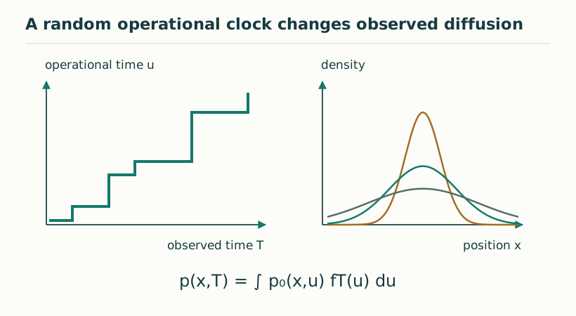
Let τ₁,τ₂,… be independent waiting times with a lower cutoff τ*. The event count N(T) is the largest n for which the first n waiting times fit within the observed interval T. Define operational time u(T)=τ*N(T). Ordinary periodic ticks would make this approximately proportional to T. Heavy-tailed waiting times produce long pauses and a different growth law. The stochastic clock is therefore a concrete object that can be simulated or measured, rather than a metaphor for vaguely irregular time.
N(T)=max{n: τ₁+⋯+τₙ≤T}
u(T)=τ*N(T)
Figure 1. A random operational clock changes observed diffusion. The illustration subordinates diffusion in operational time u to an intermittent clock u(T). Flat portions represent waiting periods. The resulting memory does not imply two independently readable laboratory clocks. View full size ↗
03The renewal scaling law
The draft chooses a Pareto density ψ_D(τ)=Dτ*ᴰτ^(−1−D), with 0<D<1. Its mean waiting time diverges, while its survival probability falls as τ^(−D). Standard renewal asymptotics then give E N(T) approximately C_D(T/τ*)ᴰ, where C_D=sin(πD)/(πD). Operational time grows sublinearly in T. The distribution and independence of increments are modeling choices; entropy maximization derives the Pareto form only after a logarithmic cost constraint has been supplied.
E N(T) ∼ C_D(T/τ*)ᴰ
E u(T) ∼ C_D τ*^(1−D)Tᴰ
04An illustrative event count
For D=1/2, C_D=2/π. At T=10,000τ*, the asymptotic mean count is approximately 63.66 events, rather than the 10,000 of a clock with exactly one τ* interval between ticks. This is an ensemble mean, not a deterministic prediction for each history. Individual trajectories can contain very long inactive stretches. A numerical study should display distributions and quantiles as well as the mean, especially because heavy tails make a single trajectory an unreliable representative of the ensemble.
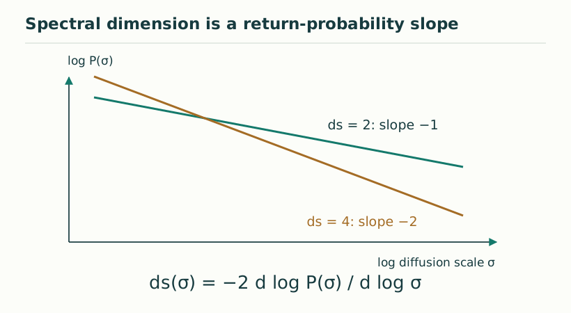
Figure 2. Spectral dimension is a return-probability slope. For the specified toy return law P(σ) = C σ⁻ᵈˢ/², the log–log slope is −ds/2. The two straight lines are ideal examples with ds = 2 and ds = 4; they are not observations of a dimensional flow. View full size ↗
05How to make the model operational
A useful completion experiment would count accepted events while independently recording outer duration. The fitted exponent should remain stable over a declared range and should be compared with exponential, tempered and correlated alternatives. A finite observation window cannot establish an infinite mean, but it can constrain a tail model. In SMM/DTT a stronger derivation would connect recurrence, retention and completion failures to this waiting law. Until then the renewal construction demonstrates how temporal intermittency can affect observations, while leaving the origin of that intermittency open.
06Why the lower cutoff is not a complete ultraviolet theory
The positive scale τ* prevents arbitrarily short waiting intervals in the chosen distribution. It sets the units of event accumulation, but it does not determine what happens during a wait, what physical state retains the pending event, or how simultaneous subsystems share the source. A simulation can sample waiting times directly; a fundamental SMM/DTT model must implement their statistics through its own retained variables and update law. One useful intermediate task is to construct a finite-state approximation with an explicit distribution of residence times and then test how its renewal law changes as the hidden state space is enlarged.
07What must be measured separately
The clock exponent D, the number of spatial coordinates, spectral dimension and a gravitational scaling dimension have different definitions. A random clock can change a diffusion diagnostic on a spatial manifold whose topology is unchanged. Similarly, an effective propagation delay is not automatically a change in a fundamental vacuum cone. A physical SMM/DTT application should identify a clock observable, state how its statistics are obtained, and compare the resulting predictions with a baseline using the same apparatus. Finite cutoffs, observation windows and normalization of probability kernels must be stated explicitly: their effects can be as important as the asymptotic power law.
Probability normalization is a practical consistency check throughout this programme. Integrating the clock density over operational time must give one at every observed time. Restoring a microscopic timescale inside a Laplace exponent can require a corresponding prefactor outside it; otherwise the averaged evolution will not preserve total probability. The same check should be made before calculating moments, return probabilities or quantum coherences. A fitted power law can look plausible even when a kernel is misnormalized, so explicit normalization is part of the derivation rather than a cosmetic convention.
KEEP THE CONNECTION
Key ideas
The random clock is specified by waiting times and accepted event counts.
Heavy tails produce sublinear mean operational time.
The clock law is an input requiring independent physical justification.
Scope of the argument. Stochastic effective model; no derivation of the waiting-time distribution from fundamental SMM/DTT axioms.
Sources & further reading
smm_dtt_fractal_time_v3.pdf — working draftpp. 3–6, §§2–4
Source editions and catalogue entries
Working manuscript
Fractal time — stochastic renewal-clock model, working draft v3
Working manuscript. Article-level references identify the consulted sections and the scope of the interpretation. No public URL was supplied for this exact manuscript version.