A return-probability slope defines a spectral diagnostic only when the return observable is finite. The inverse-stable point-return integral diverges in two or more dimensions, so the broad scaling claim needs a specified finite probe.
01A statistical realization of dual temporal roles
A diffusion probe can report an apparent dimension only when its return statistic is defined and finite. The inverse-stable clock offers an instructive test: a tempting scaling formula fails at the exact return point in sufficiently high background dimension. The calculation therefore redirects the SMM/DTT dimensional-flow proposal toward explicit detector cells, cutoffs, and reproducible finite observables.
02Define the diagnostic before interpreting it
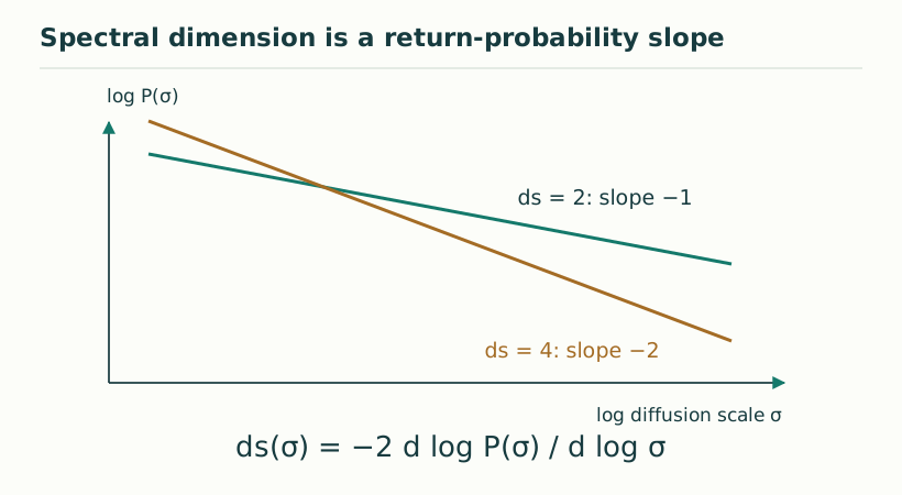
A diffusion return probability P(σ) describes how likely a probe is to return to its starting region after diffusion parameter σ. Its logarithmic slope defines a spectral dimension d_s. For ordinary Euclidean diffusion in d_E dimensions, the on-diagonal heat kernel scales as σ^(−d_E/2). This diagnostic measures diffusion and mode growth. It does not directly count axes, establish a smooth manifold, or determine how gravity scales.
d_s(σ)=−2 d log P(σ)/d log σ
Figure 1. Spectral dimension is a return-probability slope. For the specified toy return law P(σ) = C σ⁻ᵈˢ/², the log–log slope is −ds/2. The two straight lines are ideal examples with ds = 2 and ds = 4; they are not observations of a dimensional flow. View full size ↗
03The attractive scaling argument
The draft’s time-fractional diffusion equation suggests a self-similar density K_D(x,σ)=σ^(−Dd_E/2)F_D(x/σ^(D/2)), with constants absorbed into the coordinates. If F_D(0) is finite and nonzero, setting x=0 would give d_s=Dd_E. That final condition is essential. Scaling away from the origin does not guarantee that the density exists at the exact return point. The argument is therefore conditional on the chosen probe and the integrability of its return observable.
K_D(0,σ)=∫₀∞h_D(u,σ)(4πκu)^(−d_E/2)du
04The return-density obstruction
For an inverse-stable clock with 0<D<1, its density at u=0 approaches a positive quantity proportional to σ^(−D). The integral near zero therefore behaves like ∫₀ᵋu^(−d_E/2)du. It is finite only for d_E<2; it diverges logarithmically at d_E=2 and more strongly above two. Thus the draft’s unrestricted point-return argument cannot establish d_s=4D on a four-dimensional Euclidean background. This is an integrability issue in that observable, not a refutation of random-clock dynamics.
∫₀ᵋu^(−d_E/2)du < ∞ ⇔ d_E<2
05A constructive replacement
Use a finite graph, a finite spectral cutoff, or a return probability averaged over a detector cell. Each is finite and operationally definable. Then measure its logarithmic slope in a regime separated from both microscopic cutoff and finite-volume saturation, and check how that regime moves as the regulator changes. A one-dimensional background also gives a direct admissible example: the point-return integral is finite and yields d_s=D. For SMM/DTT, this more careful programme preserves the proposed temporal mechanism while replacing an overextended exponent claim with a reproducible probe-dependent calculation.
06Finite probes can exhibit a different exponent
A fixed spatial cutoff does not automatically restore the naive exponent Dd_E. With inverse-stable subordination, high-frequency modes decay algebraically in operational averaging, so the cutoff and dimension can alter the apparent return slope. The proper procedure is to compute the finite return observable itself, then vary cutoff, cell size and observation scale. A claim of universality requires a stable regime under those changes. This is why the proposed correction is more than attaching the word “regularized” to the original formula: the regulator must enter the calculation, and its removal or physical persistence must be specified.
07What must be measured separately
The clock exponent D, the number of spatial coordinates, spectral dimension and a gravitational scaling dimension have different definitions. A random clock can change a diffusion diagnostic on a spatial manifold whose topology is unchanged. Similarly, an effective propagation delay is not automatically a change in a fundamental vacuum cone. A physical SMM/DTT application should identify a clock observable, state how its statistics are obtained, and compare the resulting predictions with a baseline using the same apparatus. Finite cutoffs, observation windows and normalization of probability kernels must be stated explicitly: their effects can be as important as the asymptotic power law.
Probability normalization is a practical consistency check throughout this programme. Integrating the clock density over operational time must give one at every observed time. Restoring a microscopic timescale inside a Laplace exponent can require a corresponding prefactor outside it; otherwise the averaged evolution will not preserve total probability. The same check should be made before calculating moments, return probabilities or quantum coherences. A fitted power law can look plausible even when a kernel is misnormalized, so explicit normalization is part of the derivation rather than a cosmetic convention.
KEEP THE CONNECTION
Key ideas
Spectral dimension depends on a specified return observable.
The point-return density of inverse-stable diffusion is singular in d_E≥2.
Finite regulators or admissible probes provide constructive alternatives.
Scope of the argument. The draft’s broad d_s=Dd_E claim is qualified: its point-return derivation fails in d_E≥2 without additional regularization or probe analysis.
Sources & further reading
smm_dtt_fractal_time_v3.pdf — working draftsmm_dtt_fractal_time_v3.pdf pp. 5–8, §§4–5; integrability qualification derived here from the displayed subordinated heat-kernel integral
Source editions and catalogue entries
Working manuscript
Fractal time — stochastic renewal-clock model, working draft v3
Working manuscript. Article-level references identify the consulted sections and the scope of the interpretation. No public URL was supplied for this exact manuscript version.