A scale-dependent temporal exponent can describe a crossover without deriving its underlying clock process. A normalized kernel, integrated local slope, and regulator-dependent return calculation are needed to assess the model.
01A statistical realization of dual temporal roles
A curve interpolating between two clock exponents is a parametrization, not yet a stochastic source mechanism. This article separates that curve from a local return-probability slope and from a normalized evolution kernel. The distinctions show what an SMM/DTT model must calculate before a plotted crossover can be interpreted as generated dimensional flow.
02A crossover parametrization
The draft proposes a clock exponent that changes with diffusion scale: it approaches a short-scale value D_UV and tends toward one at large scales. A simple interpolation uses a positive crossover scale σ* and sharpness γ. It is a useful family for organizing possible data, but it does not itself specify a normalized waiting-time process with that exact running. Nor does a scale-dependent exponent inserted into a fixed-exponent formula automatically satisfy the associated evolution equation.
D(σ)=D_UV+(1−D_UV)/[1+(σ*/σ)^γ]
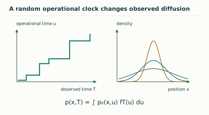
Figure 1. A random operational clock changes observed diffusion. The illustration subordinates diffusion in operational time u to an intermittent clock u(T). Flat portions represent waiting periods. The resulting memory does not imply two independently readable laboratory clocks. View full size ↗
03Local slope versus a substituted exponent
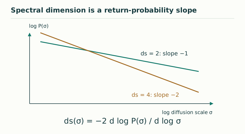
If one defines a target local spectral slope d_s(σ), the corresponding return function must be obtained by integrating that slope. Writing P(σ)=σ^(−d_ED(σ)/2) instead generates an additional term involving dD/dlogσ and logσ. The logarithm should be formed from the dimensionless ratio σ/σ*. This elementary derivative explains why a slowly varying approximation needs an explicit error regime. It also separates fitting a slope from deriving an entire probability kernel.
log[P(σ)/P(σ₀)]=−½∫_(σ₀)^σ d_s(s)dlog s
04A numerical crossover example
Choose D_UV=1/2 and γ=2. At σ=σ*, the exponent equals 3/4. At 0.1σ* it is approximately 0.505, while at 10σ* it is approximately 0.995. These values describe the chosen interpolation only. Interpreting four times these values as a measured spectral dimension requires a suitable finite return observable; the unregularized inverse-stable point kernel in four dimensions is divergent. A plotted curve should therefore identify whether it shows the clock exponent, a target slope or a computed regulator-dependent diagnostic.
Figure 2. Spectral dimension is a return-probability slope. For the specified toy return law P(σ) = C σ⁻ᵈˢ/², the log–log slope is −ds/2. The two straight lines are ideal examples with ds = 2 and ds = 4; they are not observations of a dimensional flow. View full size ↗
05How to derive rather than assume running
A microscopic model could temper long waits, mix a distribution of relaxation scales, or change completion probabilities with a controlled source parameter. Each mechanism produces a specific normalized kernel and crossover law that can be calculated before fitting. The ordinary-clock limit should be reached through such a mechanism, not by naively setting D=1 in an infinite-mean Pareto asymptotic. For SMM/DTT the central question is whether the nested source hierarchy selects one of these mechanisms and ties its parameters to independently defined records or spectra.
06One fitted curve can represent several mechanisms
A crossover in an effective exponent could arise from a tempered waiting law, a mixture of ordinary clocks, finite-size saturation or a genuine change in microscopic recurrence. These mechanisms can agree on a local slope while differing in higher moments, correlations and response to a reset. An expanded SMM/DTT study should therefore fit several observables with one clock model: event counts, waiting-time survival, diffusion profiles and coherence decay. Agreement across those quantities would constrain the source mechanism more strongly than a chosen interpolation between two attractive dimension values. It would also reveal whether the proposed running is truly slow enough for the adiabatic approximation.
07What must be measured separately
The clock exponent D, the number of spatial coordinates, spectral dimension and a gravitational scaling dimension have different definitions. A random clock can change a diffusion diagnostic on a spatial manifold whose topology is unchanged. Similarly, an effective propagation delay is not automatically a change in a fundamental vacuum cone. A physical SMM/DTT application should identify a clock observable, state how its statistics are obtained, and compare the resulting predictions with a baseline using the same apparatus. Finite cutoffs, observation windows and normalization of probability kernels must be stated explicitly: their effects can be as important as the asymptotic power law.
Probability normalization is a practical consistency check throughout this programme. Integrating the clock density over operational time must give one at every observed time. Restoring a microscopic timescale inside a Laplace exponent can require a corresponding prefactor outside it; otherwise the averaged evolution will not preserve total probability. The same check should be made before calculating moments, return probabilities or quantum coherences. A fitted power law can look plausible even when a kernel is misnormalized, so explicit normalization is part of the derivation rather than a cosmetic convention.
KEEP THE CONNECTION
Key ideas
A running exponent is initially a phenomenological parametrization.
A local slope must be integrated consistently to obtain a return function.
A finite probe and a normalized crossover clock are needed for physical interpretation.
Scope of the argument. Illustrative crossover family; no fundamental running law or unregularized four-dimensional return exponent is established.
Sources & further reading
smm_dtt_fractal_time_v3.pdf — working draftpp. 5 and 7–9, §§3.2 and 5–6; slope differentiation and integrability qualification developed here
Source editions and catalogue entries
Working manuscript
Fractal time — stochastic renewal-clock model, working draft v3
Working manuscript. Article-level references identify the consulted sections and the scope of the interpretation. No public URL was supplied for this exact manuscript version.