
The publications support conditional quotient, phase, spectral, cone and memory constructions. Later nested-stage, receiver, coupling and matter proposals must retain their own assumptions and evidence.
Read a theorem, a model and an interpretation differently
A theorem states what follows from declared mathematical hypotheses. A physical model identifies those objects with preparation procedures and measurements. An interpretation explains why that organization is meaningful. The same paper can contain all three, but publication does not make their evidential roles interchangeable.
This distinction helps answer a serious question: do the papers derive the entire SMM/DTT programme? They provide important components and explicit ways to organize further work. A claim about the universe needs the additional identification connecting each component to observable matter and clocks. The most useful reading therefore tracks the input state space, admitted operations, retained information and calibrated outputs. It asks what a result rules out within its stated class before asking how that class is physically selected.
Completion principles: a modular mathematical chain
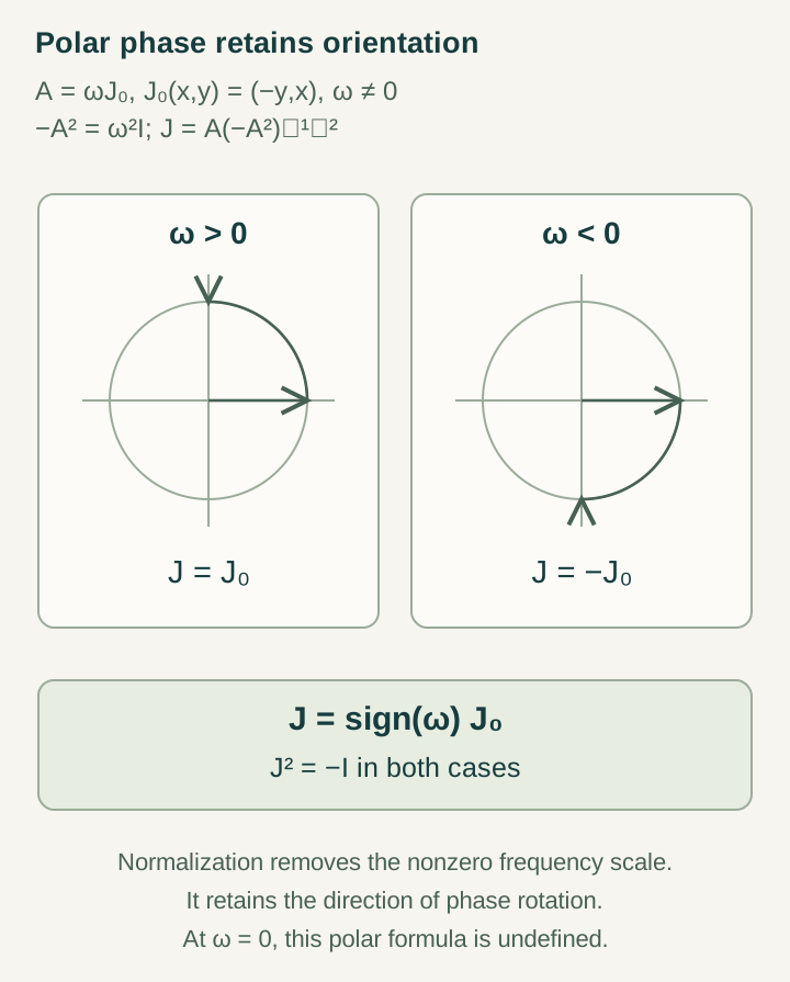
The Open Journal of Mathematical Sciences paper, volume 10, pages 996–1012, separates completed-future quotients, real orthogonal representations and downstream geometric readouts. Its representation results classify symmetry-compatible complex structures through the real commutant and select a polar phase on the nonzero-frequency sector of an oriented flow. Compact and abelian cases receive additional structural analysis.
The paper also treats phase-balanced composition and a temporal spectral-triple construction. Spectral dimension uses an explicit counting hypothesis. Its finite cone follows from supplied displacement and delay bounds; a smooth Lorentzian representative requires further geometric data. The contribution is the precise assembly and dependency bookkeeping of these modules. It does not make the length–delay interface emerge from an unspecified source merely because the earlier quotient and phase modules have been constructed.
Real-commutant phase selection: compatible phase
The Physics Letters A paper, volume 594, article 132085, addresses the selection of ordinary complex structure from real Hilbert representations. Its central distinction is between the family of phase operators permitted by the symmetry commutant and the phase selected by an oriented dynamical flow. A zero-frequency sector is not assigned an orientation by stationary evolution.
This contributes a rigorous language for obtaining quantum phase from real dynamics. It does not require a second laboratory clock, and its ordinary phase operator squares to minus identity. The split-complex unit used in hyperbolic temporal geometry squares to plus one and serves a different task. To obtain a physical quantum model, the wider programme must also identify states, available measurements, subsystem composition and their completion dynamics. Those additional interfaces should be read in their own formulations.
Open the full-size diagram →
Temporal asymmetry: geometry and projected memory
The Mathematics paper, volume 14, article 853, introduces two independent coupled temporal coordinates, connections and projection to observable evolution. Its memory representation constructs a local age-dependent field whose projected evolution reproduces a stated convolution equation. This supplies a concrete mathematical relation between an extended description and history-dependent observable dynamics.
Its geometric formulation includes ordered transport and temporal curvature. Visible consequences still depend on the projection: a transport difference acting wholly outside the accessible sector can leave the measured output unchanged. Dissipative and entropy statements use corresponding generator and functional assumptions. The published two-coordinate setting should not be silently identified with the later six nested generative roles. Establishing that identification would require a map between their states, evolution and observation rules, rather than a shared use of temporal vocabulary.
A calculation showing what a shared mechanism means
Consider the independently supplied linear example ẋ=−2x+y and ẏ=−3y+x. Integrating the second equation gives y(t)=e−3ty(0)+∫₀ᵗe−3(t−s)x(s)ds. Substitution yields a visible equation with kernel K(τ)=e−3τ and a separate initial-memory term.
The full evolution matrix has characteristic polynomial r²+5r+5, with roots (−5±√5)/2. Both are negative. This establishes decay for the example. Replacing the coefficient of y in the first equation by seven changes the determinant from five to minus one, producing one growing mode despite the same positive decay rate inside the memory kernel.
The calculation is an explanatory reconstruction, not a new theorem attributed to a journal article. It demonstrates why memory, stability and physical dissipation require separate checks. An ordinary one-time system containing x and y reproduces the same visible dynamics, so the kernel by itself does not decide between temporal ontologies.
Which constructions belong to later developments?
The paired counter, its ranks 1,1,2,2,3,3 and its 64-address/27-site example provide finite realizations of nested dependencies. Their supplied frame and pairing do the work in the rank proof. The symmetric–exterior grammar producing 137 uses additional receiver and free-retention choices. Neither result should be presented as an automatic consequence of all three published papers.
Likewise, a normalized coupling needs an energetic response and an action–clock dictionary. A Coulomb ground state follows after a Hamiltonian is supplied; matching it to hydrogen requires a physical identification. Gauge-group selection, the Pauli principle, Einstein equations and a continuum Yang–Mills gap demand their own arguments. This is a division of mathematical tasks, not a reason to abandon them. Each later construction can strengthen the programme by closing a specifically identified interface.
What is the strongest way to use the papers together?
Build one finite source with an explicitly specified retained state, oriented real evolution and completion instrument. First prove that future tests define a predictive quotient. Next verify phase selection on its dynamic sector and account for the kernel. Then measure completed displacements and delays independently and test the resulting bound. Finally compare its reduced memory with the full source evolution.
This would combine the publications through an actual common example and make unused assumptions visible. A stronger result would derive a relation among the independently defined outputs that survives changing preparation without refitting. The papers are valuable precisely because their interfaces tell the next construction what must be supplied, what can be proved and where a new physical prediction could enter.
Continue with the articles
- Completion, commutants, and positive frequency
This guide follows completion, compatible complex structures and positive-frequency selection through their separate mathematical roles. Finite examples connect the framework to SMM/DTT while keeping causal readout and physical calibration as additional constructions.
- Real-commutant phase selection: a paper guide
An oriented real orthogonal flow can select an ordinary complex structure on its dynamic sector. Planar examples explain residual zero-mode freedom, time-reversal antilinearity and the extra balancing rule needed for composite systems.
- Temporal asymmetry: reading the published model
The temporal-asymmetry model connects projected dynamics with memory and path dependence. A solvable hidden-mode example distinguishes those effects from dissipative stability and from evidence for a second observable clock.
- Six inner stages and one publication interface
A six-digit nested counter with paired signed readout realizes ranks 1, 1, 2, 2, 3, 3 before one completion interface. Its exact counts reveal sampling bias and the restricted assumptions behind the six-channel bound.
- Selecting phase by polar decomposition
Polar decomposition of an oriented real dynamical generator selects an ordinary complex structure on its nonzero-frequency sector. Zero modes, symmetry compatibility, and discrete logarithm branches remain separate inputs.
- When memory can be represented by one time
Finite auxiliary states can generate memory while evolving in one laboratory time. Rational-kernel realization identifies when that reduction is exact and which additional conditions make the auxiliary system a physical reservoir.