What would distinguish DTT from an equivalent description?

What should a distinguishing result actually compare?

Specify preparation, control sequence, clock convention, outcome registration and resources before comparing theories. Two models are operationally equivalent for a test family when every admitted protocol gives the same outcome probabilities. Their hidden variables may still differ. Conversely, a difference in internal notation or carrier dimension is not automatically a measured distinction.

The SMM/DTT ambition is to constrain geometry, clocks, matter and response through one source. It need not produce a difference in every isolated experiment. Its distinctive content may be a relationship tying several otherwise adjustable outputs together. A valid comparison holds the shared calibration fixed and identifies which remaining parameter or behavior the proposed source law forces. This is more informative than comparing a flexible model with a deliberately impoverished alternative.

Why memory alone is not a decisive signature

Let a visible variable x couple to a hidden relaxation mode y through ẋ=−ax+by and ẏ=−λy+kx. Eliminating y produces kernel K(τ)=bk e^−λτ, together with the term b e^−λty(0). Introducing y restores a first-order description using one time parameter. The two formulations predict the same outputs when their preparation data agree.

More generally, strictly proper rational transfer kernels admit finite linear state-space realizations. A nonrational pure delay excludes that exact finite class, but ordinary one-time delay equations or infinite-dimensional reservoirs remain possible. The useful DTT contribution would be a derived restriction on the kernel, its resource cost or its relation to another output. Memory’s existence is a starting measurement; the restricted joint response is the candidate prediction.

An exact test of missing predictive information

Prepare two complete states that have the same current public record. Apply the same future intervention. Suppose the probability of a binary next outcome is 0.2 in one preparation and 0.8 in the other. Any predictor using only the present record must assign one value q to both.

Otherwise both errors would be below 0.3, contradicting the triangle inequality for the separation 0.6. The midpoint q=0.5 attains the bound. This exactly excludes a record-only predictor of the declared form. It shows that completion discarded predictive information, while a larger hidden-state model can still succeed. A DTT source should calculate the two preparations and their separating intervention from its inner dynamics, rather than assume those probabilities from the desired conclusion.

Can a loop or control order reveal more structure?

For a linear prepared interface with source F, readout C, evolution A and loop operation H, the output difference after the loop is C exp(tA)(H−I)F. It vanishes if the loop fixes preparation and the relevant interface identities make its action inaccessible. Nonzero internal curvature alone is therefore insufficient.

As a concrete example take A=0, prepare the first unit vector in a real plane and read its first component. A loop rotating by θ changes the output by cosθ−1. At θ=π/3 the difference is −1/2. This supplies a visible protocol witness because the preparation is not fixed by the loop. An ordinary one-time controlled rotation reproduces it. A stronger DTT prediction would constrain this loop response together with an independently measured completion or clock quantity.

A family comparison defeats an adjustable clock label

Let independent refinement measurements give D=log B/log q and let source activities satisfy u/τ=D. Compare a protected clock T=τ with a clock T=τ+λu. Their predicted branch-to-clock conversions are D and D/(1+λD). This difference is observable once activities and clock preparation have independent definitions.

For q=2, B=4 and B=8 give D=2 and D=3. With λ=1 the conversions are 2/3 and 3/4. A single rescaling cannot make both agree with the protected values: multiplying 2/3 by three yields two, but multiplying 3/4 by three yields 9/4 rather than three. A source law selecting λ=0 across an independently defined class of clocks would therefore remove a real freedom. Merely naming the protected device the outer clock does not select it.

What should remain fixed after calibration?

Partition quantities into independent calibration inputs and held-out predictions. Among all admissible source models fitting the inputs, ask whether the proposed output is fixed or lies in a controlled interval. If it varies freely, the calculation has exposed an unfixed parameter rather than a prediction. This criterion applies equally to conventional and DTT models.

The structural receiver illustrates it. A count of 137 does not fix capacity ⟨f,K⁻¹f⟩ if stiffness K can be rescaled. A useful comparison would calibrate the source and action standard independently, then predict a response ratio, spectrum or isotope relation using the same frozen parameters. Several observables should constrain the common mechanism. Refitting the stiffness for every output would remove precisely the joint restriction the SMM programme seeks.

What would constitute a convincing advance?

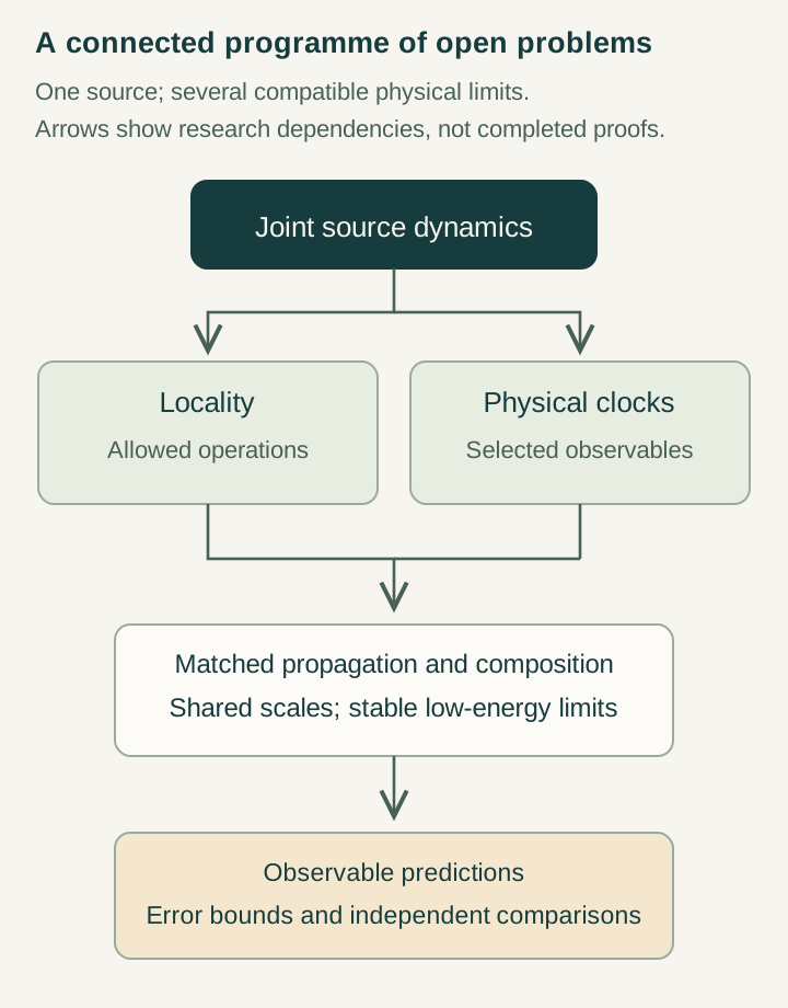
First supply a nonempty source model implementing nested generation, retained memory and a physical completion instrument. Derive a prediction for a specified protocol with an error bound and account for failed outcomes, control access and preparation resources. State the alternative class and show why its allowed parameters cannot reproduce the full predicted family after the same calibration.

A successful experimental comparison would then report measured uncertainty and the range over which the distinction survives. No such distinctive observation is asserted here. Mathematical progress can precede it: an exact witness may exclude a record-only model, while a new source theorem may remove a clock or response freedom. Each result has a precise scope. DTT gains testable content when its common-source restrictions determine something that had previously remained independently adjustable.

Continue with the articles

• Prediction after calibration

  Calibration produces a prediction only when the proposed output is fixed across the remaining admissible models, or constrained to a stated range. This criterion distinguishes cross-sector consequences from reuse of a fitted target.

• Why one clock model does not prove universality

  Protected and ungated clocks can coexist with the same record geometry while assigning different readings to it. This countermodel shows why constructing one desired clock does not establish a universal material-clock law.

• From record refinement to a joint clock–band relation

  Independent count, scale, phase, clock, and band measurements can satisfy a joint refinement relation under the supplied interfaces. The ungated-clock alternative identifies why the protected-clock premise remains essential.

• When memory can be represented by one time

  Finite auxiliary states can generate memory while evolving in one laboratory time. Rational-kernel realization identifies when that reduction is exact and which additional conditions make the auxiliary system a physical reservoir.

• Invisible holonomy in inaccessible sectors

  Parallel transport can be nontrivial in hidden sectors while acting identically on every prepared observable state. An exact intertwiner classification locates that invisible monodromy and identifies the interface assumptions an observable effect must escape.

• Empirical equivalence is not full structural equivalence

  Identical prepared behavior does not require identical full bundle structure. Concrete counterexamples separate empirical equivalence, connection-preserving trivialization and changes of the laboratory clock.

• How a protocol can reveal dual-time structure

  A temporal signature must be attached to a preparation, control sequence and readout that exposes retained information. Loop-response and predictive-state examples give exact witnesses while specifying the reduced model classes they can exclude.

• A checklist for claims of two physical times

  Claims about two physical times need operational definitions, a complete interface and an explicit comparison class. This checklist combines minimal-state reduction, memory and holonomy tests with noise-aware requirements for an observable distinction.