Can a mode count fix a normalized physical coupling?

Define the response before interpreting the count

A receiver dimension counts independent directions. A coupling describes how a calibrated source changes a measured system. To connect them, one needs a preparation, a probe, an energetic or dynamical law and a normalization standard. This is the physical bridge pursued by the normalized-coupling programme.

Let x be a real receiver coordinate, let K be a symmetric positive-definite stiffness and let f be the direction of a source with strength j. Take E(x;j)=xᵀKx/2−j fᵀx. Minimization gives x=jK⁻¹f. The measured response along f is y=fᵀx=jC, where C=fᵀK⁻¹f. Positivity ensures a unique minimum, and C is the static capacity of this specified probe.

The number of coordinates enters only through the matrix and the probe. A direction that is present but never sourced can contribute nothing; a soft direction can dominate. Thus a count becomes physically useful only after the source law fixes how the counted modes participate.

An exact two-mode counterexample

Take f=(1,1) and K=diag(2,4). Then C=1/2+1/4=3/4. Doubling K produces diag(4,8) and C=3/8. The receiver still has two modes, the source direction is unchanged and both energies are positive. Their responses differ by a factor of two.

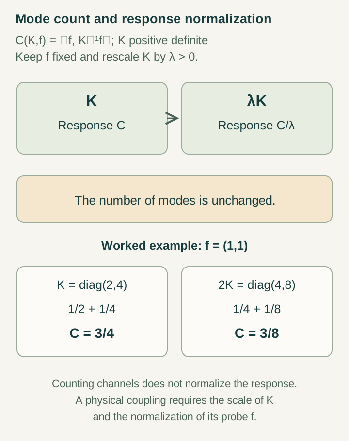
For N equal modes with K=κI and f=(1,…,1), the same calculation gives C=N/κ. If the physical observable is proportional to the inverse capacity, an inverse-rank factor appears. Its prefactor still contains κ and the units of the source and response. Calling every mode “one unit” is meaningful only after the corresponding unit is fixed by an independent physical calibration.

Why the normalization of the probe matters

The vectors f=(1,…,1) and f/√N point in the same direction but have different norms. With K=κI, their capacities are N/κ and 1/κ respectively. The first convention applies the same source amplitude to every mode; the second holds the total source norm fixed as N varies. Neither convention follows from dimension alone.

A physical trace source may select one of these conventions through a current or conserved charge. The argument must show that selection and use it consistently across receivers. Otherwise a factor of N can enter or disappear merely by changing how “equal probing” is defined. This is especially relevant when comparing the proposed 137 and 128 vacuum constructions or when translating a matrix trace into an electromagnetic source.

A reproducible response calculation should report the inner product, basis normalization, source norm and measured functional together. These data let another reader check that a purported dimensionless prediction is invariant under a change of coordinates.

Which stiffness does a visible observer actually see?

Partition the receiver into visible x and hidden z, with the positive stiffness matrix K having blocks A,B and D. At fixed x, minimization over z gives z=−D⁻¹Bᵀx and visible stiffness S=A−BD⁻¹Bᵀ. The inverse of A alone would describe a different task in which the hidden sector is held fixed.

For K with rows (2,1) and (1,2), S=2−1/2=3/2. A source coupled only to x therefore sees capacity 2/3 after relaxation; freezing z gives capacity 1/2. The full matrix is positive, with eigenvalues one and three. No instability or extra visible mode is needed for the difference. The Schur-complement guide develops this mechanism in the retained-record setting.

A source theory must decide which preparation corresponds to its vacuum response. An unobserved degree of freedom can remain dynamically relevant even when its record is absent.

What additional theorem could remove the freedom?

Symmetry can relate stiffnesses, forbid cross-couplings or select a common probe. A conservation law can identify the current. A joint matter and clock construction can determine how its action coefficient is calibrated. These are substantive mechanisms because they rule out previously admissible response matrices.

However, multiplying every allowed K by a positive scalar preserves many symmetry statements. If this transformation remains admissible after the independent calibrations are fixed, the absolute capacity remains undetermined. A useful uniqueness proof therefore studies the whole calibrated family, not just one appealing representative. It asks whether every remaining model produces the same dimensionless response.

One can first seek a ratio that cancels a genuinely common scale. If two capacities are C₁=a/κ and C₂=b/κ, their ratio is a/b. This prediction remains conditional on the same κ governing both experiments and on the coefficients a,b being fixed by independently defined probes. Such a cross-sector relation is often a more manageable first target than an absolute constant.

Does a static calibration fix the frequency dependence?

For a driven oscillator mẍ+kx=F cos(ωt), the off-resonance particular amplitude is F/(k−mω²). Its static response is F/k. Two oscillators with the same k and different m agree at zero frequency while responding differently to a time-dependent probe.

With k=4 and ω=1, masses one and two give amplitudes F/3 and F/2, although both have static amplitude F/4. This exact example identifies another source constraint: a common static stiffness does not fix the dynamical coefficient used by a physical clock or propagating probe.

A joint source programme can gain predictive force by deriving both coefficients from the same calibrated mechanism. Measuring the static response and predicting the frequency dependence would then test a relation that a mode count and a zero-frequency fit cannot establish alone. The admitted frequency range and any damping or approximation should be stated with the prediction.

What connects a capacity to an electromagnetic coupling?

A physical identification must specify the source current, matter states, propagation law and the observable used to define interaction strength. A static matrix minimum can supply part of an effective field calculation, but it does not identify charge, light propagation or an action unit by itself. The conditional ideal-value derivation exposes these remaining normalization inputs.

A non-circular test freezes those inputs using independent procedures and predicts another measurable combination. Reusing a measured coupling to set the stiffness and then recovering the same coupling from the capacity is a consistency check. Calculating a second spectrum, response ratio or preparation dependence with no new adjustment would add predictive content.

The immediate collaboration task is finite and clear: write a common source law that constrains K and f, classify its remaining allowed deformations, and show what the calibration eliminates. The outcome can be a uniqueness theorem or a counterexample. Either makes the path from a structural count to physics more precise.

Continue reading

• From record counts to a normalized physical response →
• Why a record count is not yet a coupling →
• Trace-sector response and the Schur complement →
• Open problem: fixing a normalized physical coupling →

Read this discussion as part of a path

• From structural counts to physical constants →