From retained records to normalized coupling

1. Ask a response question, not only a counting question

A retained receiver influences an interaction through the energetic cost of producing a specified output. Its number of modes tells us how many directions are available; it does not tell us how stiff those directions are, how a physical current couples to them, or how a completed field propagates between records. Those are the quantities needed to turn the structural integer into a coupling.

The SMM/DTT objective is stronger than choosing those quantities independently. The same source that prepares the records should determine their response and the matter dynamics used to measure it. This chapter identifies the exact mathematical chain and the point at which a proposed ideal normalization enters.

We begin with a finite positive quadratic model. Its assumptions are a real inner-product space of receiver fields, a positive-definite self-adjoint stiffness operator K, a fixed source direction f, and a scalar output j=⟨f,F⟩. Later steps add a spatial graph, a controlled three-dimensional continuum limit, and a matter action scale a with propagation speed c. The positive finite problem is exact; the spatial and physical matching assumptions remain explicit.

Use K for stiffness throughout. It is not the skew-adjoint time generator in the complexification chapter. Conflating the two would mix energetic cost with phase evolution before any source law has connected them.

2. Derive the constrained minimum

The receiver energy is E(F)=½⟨F,KF⟩. Fix a nonzero f and ask for the least energy among fields satisfying ⟨f,F⟩=j. Introduce a multiplier λ and differentiate E−λ(⟨f,F⟩−j). Stationarity gives KF=λf, so F=λK⁻¹f. Substituting into the constraint determines λ:

Here C is the source capacity, the response seen by this particular probe. To prove that the stationary field is the unique minimum, write any other admissible field as F*+Z with ⟨f,Z⟩=0. The cross term is ⟨Z,KF*⟩=(j/C)⟨Z,f⟩=0. The remaining excess energy is ½⟨Z,KZ⟩, strictly positive unless Z=0.

This proof does not require the receiver to be isotropic. It also shows why zero modes need separate treatment. If K is merely semidefinite, an accessible zero-cost direction can make a nonzero output free; in other cases the problem must be restricted to a supported subspace and analyzed with appropriate constraints. One cannot use K⁻¹ without checking its existence.

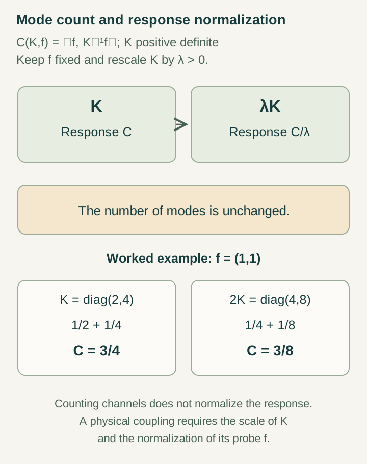
The source normalization is physical data. Replacing f by βf at fixed numerical j multiplies C by β². Replacing K by λK divides C by λ. If these are merely changes of coordinates, all related quantities must transform together; if the operational current is held fixed, they describe different response models.

3. Obtain an inverse-rank cost with ordinary trace coupling

Let the receiver field be Hermitian on an N-dimensional complex record space. Hermitian fields form a real vector space with inner product ⟨X,Y⟩=Tr(XY). Ordinary trace coupling means f=I_N, so j=Tr F. Since Tr(I_N²)=N, isotropic stiffness K=κI gives C=N/κ and E_min=κj²/(2N).

The 1/N cost reflects how an imposed trace can spread across N equally weighted diagonal directions. The minimizing field is F*=(j/N)I_N. This calculation uses ordinary trace, not normalized trace. Had the current been defined as Tr F/N, the source vector and its capacity would differ. A physical current convention must be fixed before comparing couplings.

Equal dimension does not force equal cost. Give the grammar’s sectors of sizes 100, 30 and 7 different positive stiffnesses κ₁, κ₂ and κ₃. Ordinary trace probes all of them, yielding C=100/κ₁+30/κ₂+7/κ₃. Setting κ₁=2κ and the others to κ gives C=87/κ. The count stays 137, while the response changes.

Even a symmetry argument must identify the representation on fields. Conjugation can distinguish the trace and traceless sectors, so covariance alone need not equate all of their stiffnesses. A source-derived inverse-rank law must explain both the probe and the permitted response structure.

4. Let hidden response directions relax

Normalize the identity direction as e₀=I_N/√N and decompose F=xe₀+Z, where Tr Z=0. Ordinary trace fixes x=j/√N. In this orthogonal decomposition, write K as a block matrix with scalar u, hidden vector b, and positive hidden operator D. The energy becomes ½[u x²+2x⟨b,Z⟩+⟨Z,DZ⟩].

The derivation is completion of the square: add and subtract x²⟨b,D⁻¹b⟩ to obtain ½⟨Z+xD⁻¹b,D(Z+xD⁻¹b)⟩+s x²/2. Positive definiteness of K implies positivity of this Schur complement s. Hidden relaxation lowers the cost relative to freezing Z at zero.

For u=2, D=2 and b=1 in a two-coordinate example, s=2−1/2=3/2. The relaxed field has Z*=−x/2. If the hidden mode were incorrectly clamped, the inferred stiffness would be two, overestimating the minimized cost by one third relative to its true value. This is a concrete mechanism by which inaccessible degrees of freedom affect a visible scalar response.

The scalar s summarizes a static minimization. If hidden modes relax on a finite timescale, a frequency-dependent experiment generally sees a dynamical response rather than this static number. Deriving the relaxation law and the relevant measurement regime is another way the retained-memory chapter connects to coupling.

5. Derive a graph-mediated interaction

Supply a connected finite spatial graph with one orientation per edge and incidence matrix B. Let j be edge currents and ρ be vertex sources with total sum zero. Conservation is Bj=ρ. For uniform relaxed stiffness s, the total edge energy is (s/2N)‖j‖². This graph is additional geometric input; its locality is not implied by receiver rank.

The minimum-norm conserved flow lies in the gradient subspace. Write j=Bᵀφ; conservation becomes Lφ=ρ, with graph Laplacian L=BBᵀ. Constants lie in ker L, but neutrality permits the solution φ=L⁺ρ up to a constant, using the inverse on the zero-sum subspace. Therefore:

Any other conserved flow differs by a divergence-free cycle current. Such a cycle is orthogonal to the minimizing gradient and adds positive energy. This proves the minimum and identifies the graph Green operator controlling the interaction.

Take opposite unit sources at vertices u and v. The quadratic form contains self-terms and a cross-term −(s/N)(L⁺)_uv. A potential comparison requires a declared subtraction or reference for the self-energies. On a finite graph the answer depends on geometry and boundary conditions; it is not automatically proportional to inverse Euclidean distance.

This step gives an explicit intermediate target for a source model. Construct its record adjacency, determine its conservation law, and calculate the Green operator. Only then ask which spatial limit is controlled by refinement.

6. Match the continuum coefficient and its units

Assume the graph family converges to a three-dimensional local continuum with the selected boundary condition at infinity. In the convention −ΔG=δ, the Euclidean Green function is G(r)=1/(4πr). One way to check the normalization is to integrate −∇G over a sphere: its outward flux is one. The factor 4π is therefore tied to the stated flux and area convention.

After the graph-to-continuum scaling has been derived, denote the corresponding coefficient by s_cont. Opposite unit sources then have an attractive interaction V(r)=−A_N/r, where A_N=s_cont/(4πN). The continuum coefficient includes the required cell-length and field rescalings; it cannot be equated blindly with a dimensionless finite matrix entry.

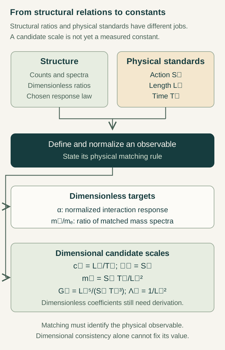
The action scale a has units of energy times time, c of length per time, and both ac and s_cont of energy times length. Their ratio η is dimensionless. A change of units changes both numerical dimensional coefficients consistently and leaves η unchanged.

Thus the ideal condition η=1 is a proposed physical relation, not a convenient choice of units. It must connect receiver response to the same action and propagation scales used by matter. Likewise, identifying g with electromagnetic α requires an identified electromagnetic current, charge normalization, and matching regime. Another mediator with the same algebraic capacity need not be electromagnetism.

7. State the ideal 1/137 claim precisely

With N=137, ordinary trace coupling, the supplied continuum limit, and the additional source normalization s_cont=4πac, the result is g₀=1/137. This is a conditional ideal-model value. It is not automatically the measured low-energy fine-structure constant, a specified bare quantum-field-theory parameter, or a running coupling at some energy.

Several changes can shift the result: a changed retained dimension, nonuniform stiffness, hidden-sector mixing, finite-resolution corrections, a different physical source normalization, or a different continuum limit. To call any of these a calculated correction, give its operator, scale dependence and effect on the measured observable.

The second line is an exact algebraic identity for the stated parametrization, not a prediction of ε. Adjusting ε after observing the desired coupling calibrates the model. The scientific question is whether the source fixes ε independently or constrains a new response once that calibration is made.

A useful local diagnostic follows by perturbing K and f. To first order, δC=2⟨δf,K⁻¹f⟩−⟨K⁻¹f,δK K⁻¹f⟩. The formula follows from δ(K⁻¹)=−K⁻¹(δK)K⁻¹. It identifies which perturbations affect the tested capacity and which are invisible at first order. Error estimates should control this sensitivity rather than assuming the finite count protects the coupling.

8. Close the loop with a matter observable

Supply the relative Coulomb Hamiltonian H=−a²Δ/(2μ)−A_N/r, with reduced mass μ. Its normalized ground state has characteristic radius a_B=a²/(μA_N) and energy E₁=−μA_N²/(2a²). The virial identity gives ⟨p²⟩/(2μ)=−E₁, hence:

This is a consistency relation between the independently defined response coefficient and a momentum statistic of the supplied atom. The stationary ground state has zero mean velocity vector. The electron’s center-of-mass RMS speed also contains the factor μ/m_e; it is not generally identical to relative speed.

Every positive g gives a bound state in this Hamiltonian. Binding therefore does not select η or N. Hydrogen becomes an independent test of source dynamics only after those inputs and the matter dictionary are fixed without using the same atomic observable as the fitting target.

9. Freeze the calibration and identify a new prediction

Let θ collect the source parameters and let A(θ) be the quantity used for calibration. The calibrated models form the set of θ satisfying A(θ)=A_observed. A second observable B is a prediction only to the extent that its value is fixed or tightly restricted across that allowed set. Merely computing A again with the fitted parameter recovers the calibration.

Concrete candidates include a nonlinear response coefficient, a frequency-dependent phase lag, a different charge sector, or an atomic transition ratio. The source should specify the preparation and measurement procedures, and the same normalization should be used across all of them. A measured difference is useful only if uncertainty from the continuum limit and parameter freedom is controlled.

The strongest common-source theorem would derive the grammar, f, K, graph scaling and matter action from one autonomous dynamics. That would reduce several choices at once. The present calculation makes this goal manageable: it identifies the primitive dimensionless ratio that remains to be selected and provides exact finite tests for every earlier step.

Sources and connected calculations

• From retained response to interaction strength: finite minimization, Schur reduction and physical coefficient conventions.
• The structural receiver derivation; the relative RMS-speed calculation.
• The normalized-coupling research target: consult the exact remaining source-selection problem.
• Completion principles, real commutants, and positive-frequency geometry for orthogonal Hilbert representations, Mohamed Haj Yousef, Open Journal of Mathematical Sciences 10 (2026), 996–1012. This publication supplies the completion/phase framework; the response chain above is the site’s explicitly conditional working construction.