SMM/DTT and empirical discrimination: SMM/DTT and Bayesian model comparison

01What data compare

Data compare probability distributions generated by models. A philosophical claim that reality has one source may allow many distributions. A particular DTT update law, preparation and readout can be much more restrictive. Success of one model supports that model under its assumptions, not every claim made within the broader programme. Bayesian inference expresses this through a likelihood and a prior over parameters. The source architecture becomes informative when it narrows the possibilities before the data are inspected. ^[1]

02What the SMM/DTT distinction contributes

SMM begins with one nonspatial generative source. DTT distinguishes its inner production from the outer order in which completed results become accessible. The six inner levels are nested functional dependencies within that production; the seventh denotes outer completion. They are not six independent clocks, six spatial directions, or six simultaneously occupied temporal axes. This distinction makes the framework more specific than a general claim that everything changes: it asks how a world of persistent relations can be generated before its spatial representation is taken for granted.

A clock is a physical system whose changes provide a reproducible comparison with other changes. Its readings are not created by writing t in an equation. Oscillations, transitions and accumulated phases become clocks when a preparation, readout and calibration connect them with a measurable interval. SMM/DTT’s distinction between generative and observed time is therefore tested conceptually by asking what an embedded clock actually counts. If an outer clock is independent of the proposed inner dynamics, their ratio remains an additional assumption.

Operational time has several layers. A counter counts events. A phase tracks periodic evolution. A calibrated clock assigns units such as seconds. A relativistic clock measures proper time along its path. These descriptions can agree in a suitable regime while responding differently to noise, acceleration or changes in the underlying state. A generative theory must recover their agreement where established physics requires it. It should also explain why different clock technologies share the same spacetime dependence, rather than assigning each species its own completion rate. ^[2]

03A complete toy Bayes factor

Consider ten independent trials producing eight successes. Model A fixes the success probability at one half. Model B fixes it at four fifths. For the same observed sequence, the likelihood ratio is (0.8⁸ × 0.2²)/(0.5¹⁰) ≈ 6.872. Equal prior odds then yield posterior odds favoring B by that factor. If B’s probability had instead been fitted after seeing the data, its evidence would require averaging over a stated prior. Fixed prediction and adjustable fit are different models. These invented trials illustrate the logic; they are not evidence for SMM/DTT.

04Why structural numbers need a bridge

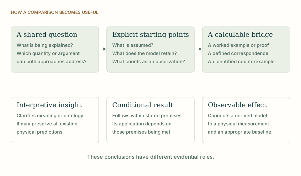
A structural label such as 137 or 128 is not yet a measured electromagnetic coupling. A model must derive a normalized response, state its vacuum and matter assumptions, and connect them with the experimental observable and scale. A fitted correction cannot retroactively turn a count into a parameter-free prediction. DTT’s opportunity is to make the bridge restrictive enough that several observables follow from the same law. Agreement then has greater evidential force because fewer independent adjustments are available.

05How the architecture can earn support

The six nested levels should exclude alternatives or impose observable relations. If any result can be reproduced by retuning hidden frequencies or changing the readout, the architecture has little discriminating content. A useful model states admissible parameters before comparison and tests consequences beyond those used to select them. A null result can rule out a model family while leaving the metaphysical motivation open. This allows progress through precise successes and failures rather than requiring one experiment to settle an entire worldview.

06A further conceptual benchmark

An oscillator with angular frequency ω accumulates phase φ = ωτ. Its inferred interval is τ = φ/ω, once ω is independently calibrated. Suppose a source completes n records and a proposed inner counter reports u = 3n. An observed ratio u/n = 3 is exact, but it contains no seconds and says nothing about the oscillator phase. To conclude that a clock ratio is three, the source dynamics must establish how φ changes with n. Two models with φ = n and φ = 2n have the same record counts and different physical timing. This counterexample shows exactly why an additional transducer law matters.

THE SAME QUESTION, DIFFERENT STARTING POINTS

The comparison at a glance

Continue on SMONAD

• Relativity and physical clocks →

  Connects this comparison with the author’s discussion of clocks.

• Limiting speed as update scale times projection rate →

  Connects this comparison with the author’s discussion of clocks.

• How a protocol can reveal dual-time structure →

  Connects this comparison with the author’s discussion of clocks.

• Relational time: order, clocks, and shared duration →

  Connects this comparison with the author’s discussion of clocks.

• A checklist for claims of two physical times →

  Connects this comparison with the author’s discussion of clocks.