Physical clocks and operational time: SMM/DTT and The thermal-time hypothesis

01The question behind the comparison

A clock is a physical system whose changes provide a reproducible comparison with other changes. Its readings are not created by writing t in an equation. Oscillations, transitions and accumulated phases become clocks when a preparation, readout and calibration connect them with a measurable interval. SMM/DTT’s distinction between generative and observed time is therefore tested conceptually by asking what an embedded clock actually counts. If an outer clock is independent of the proposed inner dynamics, their ratio remains an additional assumption.

Operational time has several layers. A counter counts events. A phase tracks periodic evolution. A calibrated clock assigns units such as seconds. A relativistic clock measures proper time along its path. These descriptions can agree in a suitable regime while responding differently to noise, acceleration or changes in the underlying state. A generative theory must recover their agreement where established physics requires it. It should also explain why different clock technologies share the same spacetime dependence, rather than assigning each species its own completion rate.

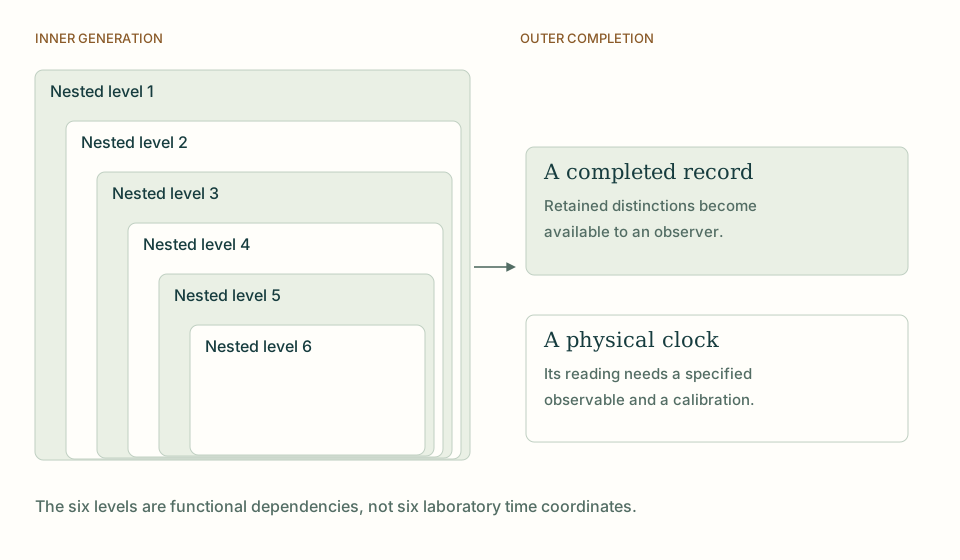
The six nested levels are not six separate clocks that can be adjusted until a desired ratio appears. Their proposed role is to organize how a completed state becomes available. A successful clock law would derive a phase or counter response from that same source trajectory. Changing a refinement or branching parameter would then change geometry and timing in a linked way. If the oscillator frequency is retuned whenever the geometry changes, a numerical agreement demonstrates calibration freedom rather than a necessary physical relation. This is the decisive distinction between a constructive explanation and a convenient parametrization.

02The single-source and nested-time proposal

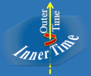
SMM begins with one nonspatial generative source. DTT distinguishes its inner production from the outer order in which completed results become accessible. The six inner levels are nested functional dependencies within that production; the seventh denotes outer completion. They are not six independent clocks, six spatial directions, or six simultaneously occupied temporal axes. This distinction makes the framework more specific than a general claim that everything changes: it asks how a world of persistent relations can be generated before its spatial representation is taken for granted. ^[2]

03The comparator’s explanatory structure

Connes and Rovelli propose that an algebra of observables together with a state can determine a temporal flow. In a finite faithful-state illustration, write K = −ln ρ and let observables transform as A(s) = exp(isK)Aexp(−isK). The parameter s is dimensionless. If ρ is a Gibbs state proportional to exp(−βH), then K differs from βH only by a scalar, so s can be related to ordinary Hamiltonian time by t = ℏβs in this convention.

This example explains both the power and the limitation of the comparison. Time need not be an independently supplied universal background, but the observable algebra and state are already doing essential work. A maximally mixed finite state gives a scalar K and hence trivial flow on that full matrix algebra. Different physical states can therefore select different flows. The thermal-time programme is not a claim that every microscopic event dissipates heat, nor does modular evolution alone constitute a thermodynamic arrow. DTT asks the further question of how the relevant state, algebra and accessible records are generated. ^[1]

04The precise agreement and difference

Thermal time supplies a candidate flow from a state, but a physical clock must still be coupled and calibrated to that flow. In the Gibbs example, the relation t = ℏβs depends on inverse temperature β and the Hamiltonian convention. The dimensionless modular parameter is not automatically a universal second. DTT faces the analogous requirement when converting completion counts into outer duration.

The strongest bridge would derive both the accessible state and the clock’s response from one source trajectory. It would then explain why the clock tracks the selected modular flow in a specified regime. A useful failure case is a maximally mixed finite state, whose modular action is trivial on the full matrix algebra: a nontrivial oscillator cannot be identified with that flow without changing the setting. This comparison gives DTT a rigorous target and a diagnostic counterexample. The six nested levels matter if they select the observable algebra, state and transducer relation together, not if they simply provide enough adjustable frequencies to reproduce a chosen clock ratio. ^[1]

05Worked example: what follows and what does not

An oscillator with angular frequency ω accumulates phase φ = ωτ. Its inferred interval is τ = φ/ω, once ω is independently calibrated. Suppose a source completes n records and a proposed inner counter reports u = 3n. An observed ratio u/n = 3 is exact, but it contains no seconds and says nothing about the oscillator phase. To conclude that a clock ratio is three, the source dynamics must establish how φ changes with n. Two models with φ = n and φ = 2n have the same record counts and different physical timing. This counterexample shows exactly why an additional transducer law matters.

06What this comparison contributes

A promising DTT explanation therefore uses clocks as outputs of the same theory that produces spatial relations. The result should be robust under changing the way a calculation is labelled and should state its domain of approximation. This operational standard does not diminish the philosophical distinction between production and observation; it gives that distinction a concrete route into physics. The most informative comparison asks which theory supplies the clock, which merely orders events, and which leaves the conversion from order to duration open.

THE SAME QUESTION, DIFFERENT STARTING POINTS

The comparison at a glance

Continue on SMONAD

• Relativity and physical clocks →

  Connects this comparison with the author’s discussion of clocks.

• Limiting speed as update scale times projection rate →

  Connects this comparison with the author’s discussion of clocks.

• How a protocol can reveal dual-time structure →

  Connects this comparison with the author’s discussion of clocks.

• Relational time: order, clocks, and shared duration →

  Connects this comparison with the author’s discussion of clocks.

• A checklist for claims of two physical times →

  Connects this comparison with the author’s discussion of clocks.