Three-dimensional readout: from source algebra to spatial geometry

1. The precise question and its assumptions

Why should a common generative process have a three-dimensional public readout? The Single Monad Model makes the unity of generation a guiding premise; the Duality of Time Theory distinguishes inner generative organization from completed, available records. Neither premise alone assigns a dimension. A useful reconstruction must name its carrier, operations, detector family and completion rule, then calculate which distinctions survive. This chapter follows two explicit routes to rank three and identifies the further work required for physical space.

The first route assumes a finite-dimensional real unital associative algebra with a positive-definite inner-product norm that is multiplicative, and two noncommuting elements whose squares equal −1. It also assumes that the joint linear detector family ignores exactly the real scalar direction. The second route supplies six paired channels in a three-vector frame. These are different input packages. Agreement of their output dimensions is a candidate connection to explain, rather than an identification already licensed by dimensional counting.

Keep four questions separate throughout: what composes in the source; what an observer can distinguish; how records are connected and compared; and how signals and clocks evolve. A theorem at the first two levels can be exact while the latter two remain open. The source and retained-memory chapter develops the completion interface needed to relate them.

2. Select the algebra before counting directions

Let the algebra be A and its norm N satisfy N(ab)=N(a)N(b), with N(a)>0 for every nonzero a. If ab=0 and a,b are nonzero, multiplicativity gives 0=N(a)N(b)>0, a contradiction. Thus there are no nonzero zero divisors. For fixed nonzero a, left multiplication L_a is injective. In finite dimension it is surjective, so there is b with ab=1. The analogous argument gives c with ca=1. Associativity then gives c=c(ab)=(ca)b=b: the two inverses agree.

Consequently A is a finite-dimensional associative real division algebra. The classical classification leaves ℝ, ℂ and ℍ. Noncommuting circular phase elements exclude the first two, selecting the quaternion algebra within this stated class. Dropping associativity, positivity or finite dimension changes the classification problem; none of those assumptions can be silently removed from the conclusion.

The four coefficients describe a compositional carrier. They do not yet describe four locations, four spacetime coordinates or four independent time readings. In particular, the scalar coefficient can participate in multiplication even if a spatial detector subsequently ignores it. This distinction is essential to the SMM/DTT interpretation: generation can carry information that a completed geometrical output does not display.

3. Compute the scalar-insensitive quotient

Define the imaginary projection π(q)=xi+yj+zk. Its kernel is ℝ1 and its image is Im ℍ. The first isomorphism theorem for real vector spaces gives a three-dimensional quotient. The word “linear” matters here: ℝ1 is not a two-sided ideal of ℍ, since multiplying 1 by i produces i outside ℝ1. There is no induced quaternion multiplication on this quotient merely from identifying scalar shifts.

A norm on a coset is obtained by minimizing over its scalar representative. For q=a+v, the squared norm of q+b is (a+b)²+|v|²; its minimum occurs at b=−a. The quotient norm is therefore |v|. The inner product on the imaginary sector can also be recovered algebraically: for imaginary v,w, their product has scalar part −v·w and imaginary part v×w.

For q=2+3i−4j+12k and q′=7+3i−4j+12k, both outputs are (3,−4,12), of norm 13. Their full squared carrier norms are 173 and 218. The same public vector can therefore coexist with different source information. A supplied length unit ℓ gives length 13ℓ; the quotient itself does not calibrate metres.

4. Make three directions operationally accessible

A scalar-insensitive detector need not read the entire quotient. The map D(a+xi+yj+zk)=x satisfies D(q+b)=D(q), but it sees only one component. For a collection of linear tests D_r, complete access means that their joint kernel is exactly ℝ1. Equivalently, their restrictions to Im ℍ span the three-dimensional dual space. This criterion identifies the information available through a family of experiments rather than treating algebraic coordinates as automatically observed.

Unit quaternions act by v↦uvu⁻¹. The scalar part remains zero and the norm is unchanged. For u=cos(θ/2)+k sin(θ/2), direct multiplication gives i↦cosθ i+sinθ j and j↦−sinθ i+cosθ j, while k is fixed. An accessible rotation followed by a fixed nonzero directional detector can therefore read a different component.

For example, the x detector reads x directly, reads −y after a positive quarter-turn around k, and reads z after a suitable quarter-turn around j. Correcting the known signs recovers the vector. The required control operations must actually belong to the source protocol. A pair of isolated half-turns can leave an axis inaccessible; merely possessing two quaternion symbols does not provide all continuous rotations. DTT completion must specify when these tests are executable and when their outcomes become retained records.

5. Calculate the stability of dimension

Exact rank can hide poor experimental access. Let the first phase direction be i and the second be u=ηi+s j, where s=√(1−η²) and |η|<1. Their product is iu=−η+s k. Measure projections onto i, u and Im(iu). In the orthonormal basis (i,j,k), the acquisition matrix M has rows (1,0,0), (η,s,0) and (0,0,s). It sends the unknown vector v to three readings.

The smallest singular value is √(1−|η|). If measured data are Mv+δ with error norm at most ε, reconstruction by M⁻¹ has error at most ε/√(1−|η|). For η=3/5, the three squared singular values are 2/5, 8/5 and 16/25. An input error bound of 0.01 then gives a reconstruction bound of approximately 0.01581 in the same units.

As the two phase directions approach alignment, the determinant stays nonzero until the endpoint but error amplification diverges. A persistent three-dimensional readout needs a lower bound on this singular value over the relevant source evolution. Renormalizing the weak third detector does not remove the physical issue: it also magnifies its raw measurement noise and control cost. A source-level dimensional theorem should therefore report both rank and conditioning.

6. Relate phase-bearing spinors to directions

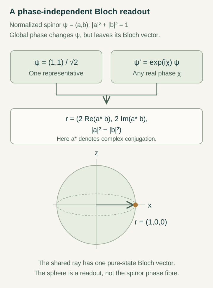
Choosing an ordinary complex slice of ℍ gives a representation by two complex components. For a normalized doublet z=(z₁,z₂), define n=(2Re(z₁* z₂),2Im(z₁* z₂),|z₁|²−|z₂|²). The first two squared components sum to 4|z₁|²|z₂|². Adding the third gives (|z₁|²+|z₂|²)²=1. Thus the readout lies on a sphere.

The global phase cancels because z₁* z₂ is unchanged, as are both squared magnitudes. The domain of normalized doublets is S³; the phase fibres are circles. This is the familiar Hopf relation between phase-bearing data and direction. It complements the linear quotient, but it is not that same quotient: removing an additive real scalar from ℍ and identifying common complex phases of normalized spinors are different operations on different domains.

The Bloch sphere describes pure-state directions of a supplied doublet. It is not a sphere of physical positions. To identify its axes with spatial rotations one needs the corresponding representation of actual preparation and detector operations. To identify the doublet with matter one further needs propagation, coupling and state interpretation. The complexification chapter explains how a compatible phase can be selected before those additional physical identifications.

7. Compare the six-role paired construction

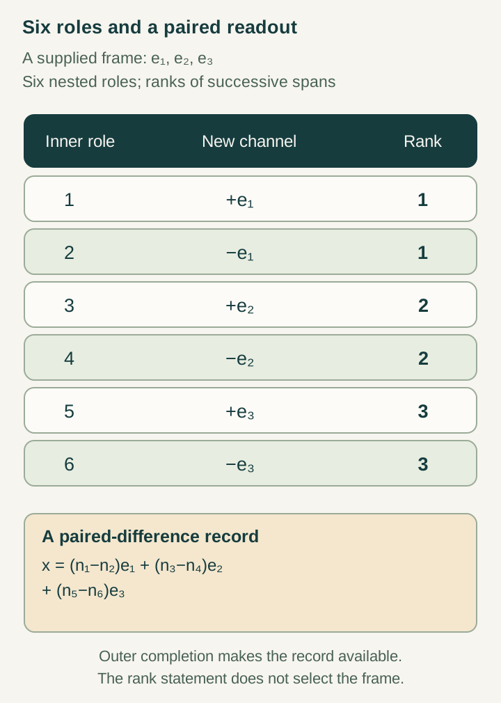
A second finite model starts with six digits d_a∈{0,…,q−1}, q≥2, ordered by the single counter n=Σq^a−1d_a. One elementary update is n↦n+1 modulo q⁶. Supply three independent vectors e₁,e₂,e₃ and a positive scale ℓ. The proposed display is Q(d)=ℓ[(d₁−d₂)e₁+(d₃−d₄)e₂+(d₅−d₆)e₃].

Starting from zero, the first q^a addresses vary exactly the first a digits. Their image lies in the span of the first a signed columns, giving rank at most ceiling(a/2). Conversely, zero and each available single odd-digit address occur in that prefix. Their images include ℓe₁, then ℓe₂, then ℓe₃, proving the matching lower bound.

The digits have nested carry dependencies, not six independently adjustable clocks. If primitive channels are exchanged in opposite pairs by an involution P and a linear readout C satisfies CP=−C, the even eigenspace is invisible. Each exchanged pair supplies one odd direction, so rank C≤number of pairs. Six channels are minimal for rank three within this architecture. Three initially signed coordinates, or four nonnegative-weight channels along tetrahedral directions, use different architectures and evade that bound.

For q=2, 64 addresses collapse to 27 displayed sites. Each coordinate difference has multiplicities 1,2,1 at −1,0,1, so the central site has eight preimages and a corner has one. Uniform source sampling therefore does not give uniform spatial measure. The binary derivation computes the induced measure. Linking this paired readout to the quaternionic quotient requires a common source construction that selects both maps, not simply a change of labels between two three-dimensional vector spaces.

8. Check whether the readout predicts its own future

An instantaneous spatial quotient can fail to support autonomous evolution. The descent test is simple: whenever Q(x)=Q(y), must Q(Tx)=Q(Ty)? If it fails, there is no single-valued map on displayed vectors representing the elementary source update. One must retain additional memory, change the completion boundary, or describe the display through a history-dependent process.

The paired counter supplies a concrete failure. Addresses n=0 and n=q²−1 both display zero: the latter has d₁=d₂=q−1 and all higher digits zero. But their successors display ℓe₁ and ℓe₂ respectively. The carry state invisible in the present vector changes the next observed direction.

This example explains why source state size, spatial rank and retained predictive memory should not be collapsed into one number. Spatial detectors can legitimately forget a scalar or carry, while a complete predictive record must keep whatever future tests can recover. The same issue can arise for quaternionic readouts if multiplication converts a previously hidden scalar component into a visible imaginary component. A completion protocol must demonstrate descent for its actual operation family or explicitly retain the missing distinctions.

9. Build locality and distance from record comparisons

Three distinguishable components do not define which records are neighbours. Supply a connected graph whose vertices are completed records and whose edges represent allowed elementary comparisons. Assign each edge e a positive length ℓ_e. For an observable f on vertices, represent its two endpoint values diagonally on an edge block and take D_e=ℓ_e⁻¹[[0,1],[1,0]]. A direct sum over edges gives the exact comparison seminorm below.

Every allowed f changes by at most the sum of edge lengths along any path, so d is at most shortest-path distance. Conversely f(z)=dist(z,y) changes by at most ℓ_e across each edge and attains the shortest-path value between x and y. This proves equality. With edge lengths AB=2, BC=3 and AC=7, the distance AC is five, achieved by f(A)=0,f(B)=2,f(C)=5. Shortening AC to four changes that distance to four without changing the readout’s vector-space dimension.

A cubic lattice with only axial unit edges has Manhattan distance. The separation from (0,0,0) to (1,1,0) is two, not √2. Refining that same path-cost rule does not itself produce a Euclidean norm. An isotropic limit requires justified additional comparison directions or a different effective probe law. Likewise, a graph that looks local in a drawing does not force its dynamics to be local.

If each update layer is a product of gates with pairwise disjoint supports, each of graph diameter at most R, conjugating a local observable through n such layers expands its support by at most nR in graph distance. That is a separate finite-support theorem under a supplied circuit architecture. The source must explain the edges, their lengths, the update supports and their stability together. The metric guide and locality guide give the individual proofs.

10. Derive a cone and state its clock dependence

A positive two-by-two Hermitian record can be written X=T I+x·σ, using the Pauli matrices. Their anticommutation relations imply (x·σ)²=|x|²I, so X has eigenvalues T±|x|. Consequently X≥0 exactly when T≥|x|, and det X=T²−|x|². This is a round future-cone shape in the four-dimensional space of Hermitian matrices.

The algebraic coordinate T is not automatically a reading on a material clock. A physical identification needs T=cΔt with units and calibration specified. An alternative finite-transition route assumes a path-length budget ds≤κdθ and a physical clock law dt=dθ/ρ, with κ,ρ>0. Summing or integrating yields Δs≤κρΔt. For κ=2 and ρ=3, four activity units permit at most eight length units in 4/3 clock units, giving a speed bound of six.

The product c=κρ is fixed by that ratio, but the factors are not separately identified by measuring c. Scaling κ by b and ρ by 1/b leaves the bound unchanged. A clock/cone derivation becomes informative when those two ingredients have independent operational definitions and follow from the same dynamics. A positive delay on every edge also need not define a global event-time function: delays must sum consistently along alternative paths, and a directed positive-delay cycle obstructs an exact global clock.

11. What turns the readout into physical spacetime?

A smooth four-dimensional description requires more than adding a time label to three vector components. Completed events must organize into a stable local structure; a clock one-form and spatial comparison frame must be independent; and an invertible identification with tangent directions must be justified. Once those inputs exist, a coframe (θ,e¹,e²,e³) defines a candidate metric g=c²θ⊗θ−Σe^a⊗e^a. Its Lorentzian signature follows from coframe independence, not from the bare number of source symbols.

A cone fixes less than a metric scale. Replacing g by Ω²g, Ω>0, preserves null directions. Operational volume or clock normalization must fix the additional information. More importantly, the characteristics of actual matter and electromagnetic equations must agree with this cone. One can place two wave equations with different propagation speeds on the same manifold; a geometric drawing alone does not prohibit the mismatch.

The SMM/DTT target is therefore joint: derive an accessible spatial comparison, a reproducible clock and a transport law from one source update, then prove their agreement without defining one from the others. Such a result would connect the exact readout calculations to relativity. It would still need separate treatment of interaction strengths and bound matter. The normalized-coupling chapter and hydrogen chapter make those dependencies explicit.

12. A concrete research programme and reading route

Begin with a finite model in which all admissible source operations are listed. Compute the joint detector kernel and smallest singular value. Verify whether the completed update descends; if it does not, enlarge the retained record until the missing predictive distinctions are explicit. Next generate a comparison graph, calculate its metric and support-growth bound, and repeat these tests across refinement levels with fixed landmark records.

Independently construct a material clock observable and a signal preparation. Compare measured completion delays with graph distances and the proposed cone coordinate. A useful error statement would bound spatial reconstruction error, clock drift and leakage outside the nominal propagation region with the same finite resource budget. Persistent disagreement is evidence against the selected interface, even when its algebraic rank remains three.

The published completion and positive-frequency paper (DOI 10.30538/oms2026.0328) supplies a modular setting for observable descent and conditional cone readouts. Its cone result requires supplied length-delay data. The quaternionic and paired-channel calculations above are explanatory reconstructions developed in this site’s three-dimensional-readout guide and paired-rank derivation; they should not be attributed to that paper as an unconditional spacetime theorem.

Proceed to the structural-count chapter to see why selecting a carrier and a readout does not yet select a receiver grammar. A dimension is a precise result about an object. The larger explanatory advance comes when one justified source law constrains which object, which accessible tests and which physical dynamics occur together.