
Counting exponent, metric distance, and locality must be established separately, then related through a common source-generated algebra and operator.
The preprint and the reconstruction target
Non-Commutative Geometric Foundations for the Emergence of Spatial Dimensions and Physical Structures from Complex-Time Spectral Triples is a public preprint. Its abstract proposes hierarchical temporal compactification and a spectral account of emergent structure. This guide develops a reading test for those proposals, extending A211.
Three statements can sound similar while proving different things: a carrier has three independent directions; an eigenvalue count grows cubically; or accessible records form a space with local three-dimensional metric behavior. An argument must state which result each calculation delivers.
Count an explicit family of modes
Take nonnegative integers n₁,n₂,n₃ and positive weights ω₁,ω₂,ω₃. The region ω₁n₁+ω₂n₂+ω₃n₃≤Λ is a tetrahedron in mode-index space. Its continuum volume is Λ³/(6ω₁ω₂ω₃), giving the leading lattice-count growth at large Λ.
The cubic exponent follows from the three independent supplied indices. This is a useful exact asymptotic target for a source model, but changing the number of indices changes the exponent. A derivation of dimensional selection must explain why the underlying carrier has this index structure.
Ask what a detector can distinguish
Suppose records carry labels (x,y,z), but every admitted detector function depends only on x and y. The accessible spatial quotient identifies all records with the same pair (x,y), irrespective of z. A three-entry label has then produced only two distinguishable directions for that interface.
If later transport allows a z-dependent effect to reach the detector, that reduced quotient is no longer predictively sufficient. Observable dimension must therefore be assessed against the chosen test family and its future continuations. The structure of a source carrier and the structure of its public records can differ.
Show how a relation becomes a distance
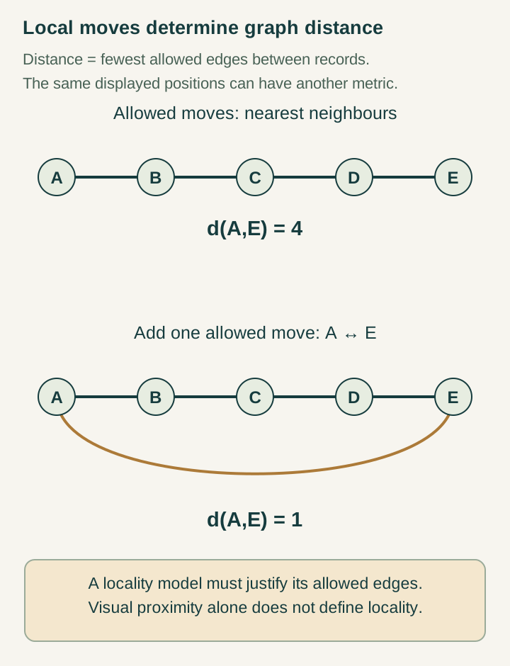
For a finite chain of records, assign a positive cost to each allowed neighboring transition. A path cost is the sum of its edge costs, and distance is the least such cost. Positivity and connectedness ensure finite distances; reversing edges with the same costs gives symmetry.
Those conditions are inputs until the source creates them. A spectral operator can encode the same comparisons, but the commutator bound must actually reproduce finite distances on the intended states. Merely matching the mode-count exponent does not establish this. The two-point calculation in the noncommutative guide is the smallest illustration.
Open the full-size diagram →
Locality must persist under evolution
A graph can have recognizable neighborhoods while its dynamics jumps arbitrarily between distant vertices. Conversely, a local dynamics can be programmed on a graph without explaining why that graph was selected. Formation, selection, and persistence are therefore separate tasks.
SMM asks one source to generate the relations. DTT organizes their nested construction and completed publication. The rank sequence 1,1,2,2,3,3 is a candidate organization of readout roles; it does not by itself supply a metric, a probability favoring local graphs, or a transport Hamiltonian respecting their neighborhoods.
A three-column audit
Read A211 together with A155–A157 and A123–A128. For each claimed geometry, make three columns: spectral count, operational distance, and allowed propagation. Write a concrete definition and a verified result in every column before joining them.
The strongest next finite example would derive the graph, the normalized spectral operator, and the transport rule from the same retained-history update. Which locality property survives repeated completion? Does a controlled large-system limit produce stable metric behavior? These questions turn the claim that time creates space into a sequence of measurable and reproducible constructions.
Continue with the articles
- Spatial dimensions from spectral triples: a guide
A three-dimensional mode count, metric distance and stable local space are different reconstruction targets. Explicit counting and graph examples identify the observable algebra and dynamical selection needed to connect them.
- Three-frequency counting and inner spectral dimension
Three supplied frequency labels yield cubic eigenvalue growth, even with anisotropic weights. Adding an independent outer Fourier label changes the count, and neither exponent alone determines physical distance.
- Why spectral dimension does not determine distance
An operator can have cubic spectral growth while assigning infinite distances between localized evaluation states. The counterexample shows why record comparisons require commutator control beyond mode counting.
- Graph distance from a normalized spectral block
A direct sum of normalized edge blocks gives a commutator seminorm equal to the largest edge slope. Its state distance is exactly weighted shortest-path distance on a connected finite graph.
- Why local geometry can be statistically rare
Lattice-like signed operation tables are rare in the stated permutation ensemble, with an entropy penalty of order N log N. Bounded selection costs cannot overcome that asymptotic disadvantage under the theorem's assumptions.
- Six inner stages and one publication interface
A six-digit nested counter with paired signed readout realizes ranks 1, 1, 2, 2, 3, 3 before one completion interface. Its exact counts reveal sampling bias and the restricted assumptions behind the six-channel bound.
- Generating a neighborhood and preserving local transport
A generated graph predicts local influence only when later operations respect its edges and retained ports. Guarded transport supplies a finite-update support bound while exposing runtime and controller-memory requirements.
- What spatial readout forgets
Different inner states can share one spatial readout and still have different successors. A concrete counterexample and a kernel-preservation criterion identify the memory needed for autonomous completed evolution.
Sources and reading
Read the original source for its exact formulation and edition. The examples on this page are explanatory reconstructions.