
Polar decomposition selects a unique quarter-turn on the dynamic sector. Positive Schrödinger evolution uses i=−J; shared phase in a composite is then enforced by a distinct balancing construction.
1. Start with a real carrier and an actual evolution
Let V be a finite-dimensional real inner-product space. Choose a real linear generator A with Aᵀ=−A and define U(t)=exp(tA). These are the inputs: a carrier, an inner product, a dynamics and its orientation. The equation ẋ=Ax does not initially require multiplication by an abstract imaginary scalar.
Differentiating U(t)ᵀU(t) gives U(t)ᵀ(Aᵀ+A)U(t)=0. Because U(0)=I, the flow preserves the norm. Thus a skew generator supplies reversible rotations on real planes. Its time parameter still requires an operational clock if it is to represent a measured physical duration.
The reconstruction asks whether this dynamics selects an operator that behaves as multiplication by i. A suitable operator must satisfy J²=−I and preserve the real norm. Such a J turns an even-dimensional real space into a complex space by declaring (a+ib)x=ax+bJx.
This ordinary complex structure differs from the split-complex temporal unit j satisfying j²=+1. The latter produces hyperbolic algebraic relations; the former produces circular phase. They cannot be interchanged by a change of lettering. In SMM/DTT they may describe different roles of a construction, but an explicit map is needed before one can claim they follow from the same source operations.
2. Derive the selected phase by polar decomposition
First assume A is invertible. Since Aᵀ=−A, the matrix −A²=AᵀA is positive definite. For every nonzero x, its quadratic form equals ‖Ax‖²>0. Let Ω=(−A²)1/2 be its unique positive square root. Spectral functional calculus, or the real rotation-block decomposition, shows that Ω commutes with A.
Define J=AΩ⁻¹. Commutation gives J²=A²Ω⁻²=−I. Transposition gives Jᵀ=−J, and consequently JᵀJ=I. Finally A=JΩ. The factor Ω contains the positive magnitudes of the rotation rates; J contains their orientation.
Uniqueness follows from the positive polar decomposition. If A=KB with K orthogonal and B positive definite, then AᵀA=B², so B=Ω and K=J. The conclusion is stronger than saying that some imaginary-unit operator exists: the supplied oriented flow selects this one.
If a real symmetry R commutes with A, then it commutes with −A² and its spectral functions, hence with Ω and J. Therefore the selected phase belongs to the commutant of the source symmetries. That is the link to the cited real-commutant papers. The finite proof here establishes the construction directly, without extending inverse formulas to unbounded operators or unspecified domains.
3. Work through two frequencies and one stationary direction
On a plane define J₀(x,y)=(−y,x). For A=ωJ₀ with ω≠0, the positive magnitude is Ω=|ω|I and the selected factor is J=sgn(ω)J₀. Normalization removes the rotation speed while retaining its orientation.
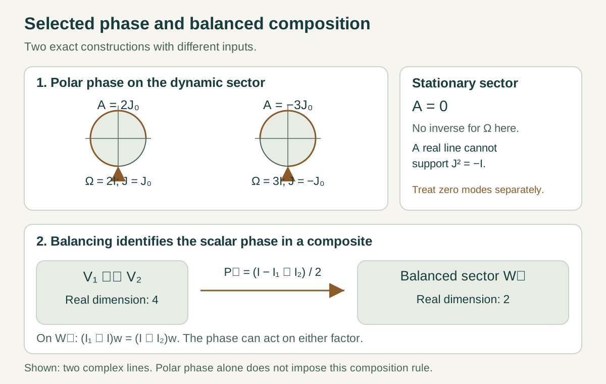
On four real coordinates take A=diag(2J₀,−3J₀) in chosen inverse-time units. Then Ω=diag(2I,3I) and J=diag(J₀,−J₀). Both blocks satisfy J²=−I even though they rotate with different rates and opposite orientations. Their exact flows are exp(tωJ₀)=cos(ωt)I+sin(ωt)J₀.
Append one stationary real coordinate. The new generator has a kernel, so Ω⁻¹ does not exist there. The dynamic orthogonal complement of ker A remains invariant and supports the construction above. The stationary line cannot carry a real J squaring to −I, because a real scalar cannot square to −1. Appending a stationary plane permits a complex extension but does not select its orientation.
Thus a zero-frequency sector is not a harmless missing denominator. It changes the question from a unique phase on the dynamic space to existence and choice of a global extension. In a physical source model, the state space of retained records may include such stationary sectors even when the inner generator is nontrivial elsewhere.
4. Obtain positive Schrödinger form without hiding a sign
The real evolution is ẋ=JΩx. Introduce a positive action scale a and let H=aΩ. To match the conventional equation i aψ̇=Hψ with the same forward flow and positive H, represent complex multiplication by Ic=−J. Then:
Equivalently exp(−IcHt/a)=exp(tJΩ)=U(t). If one instead chooses i=J while leaving the forward flow unchanged, the corresponding Hamiltonian is −aΩ. Both conventions are mathematically consistent; mixing the positive Hamiltonian of one with the scalar orientation of the other is not.
With the inner product convention linear in the second argument, the reconstructed Hermitian form is h(x,y)=⟨x,y⟩+i⟨Icx,y⟩. Indeed h(x,Icy)=ih(x,y), using skew-adjointness and Ic²=−I, while h(x,x)=‖x‖². This makes the Hilbert-space interpretation explicit.
The scale a has dimensions of energy times time. Ω has inverse-time units only after a physical time calibration is fixed. Multiplying a and H by the same positive constant leaves H/a, and therefore the flow, unchanged. The polar theorem cannot remove that freedom. Setting a=ħ recovers the usual physical conversion but does not derive Planck’s constant. A source derivation needs an independently defined energy resource and a law fixing its relation to the measured clock.
5. Derive an observable phase difference with a supplied instrument
Use the two dynamic complex lines of the example and prepare the normalized state ψ(0)=(1,1)/√2 in their positive-energy convention. With H=a diag(2,3), evolution gives ψ(t)=(e−2it,e−3it)/√2. Let the detector project onto |+⟩=(1,1)/√2.
Supplying the usual quantum probability rule gives:
The response depends on the frequency difference, which is one in the chosen units. A common energy shift H↦H+E₀I multiplies the entire state by a common phase and leaves this probability unchanged. The experiment measures relative phase, not the absolute orientation of a single unobserved rotating vector.
This is a complete worked model once the preparation and projector are admitted. Those operations do not follow merely from Aᵀ=−A. A source account should derive why its completion interface implements this detector, which states can be prepared and which coherence survives until the record is read.
The example also distinguishes structural reconstruction from empirical novelty. Rewriting a familiar two-level quantum system in real coordinates gives equivalent predictions. A new DTT prediction would require an additional, source-derived restriction on the generator, instrument or allowed preparations that cannot be removed by an equivalent reformulation. Such a restriction should affect several related measurements with fixed parameters.
6. Prove the balancing construction for two carriers
Suppose two real spaces V₁,V₂ carry selected imaginary-unit operators I₁,I₂. Their real tensor product has dimension 4n₁n₂ when the factors have complex dimensions n₁,n₂. The intended complex tensor product has real dimension only 2n₁n₂. Independent phase selection has therefore not yet determined composition.
On W=V₁⊗ℝV₂ define L=I₁⊗I₂. Since each I squares to −I, L²=I. Since both are skew-adjoint, L is self-adjoint. Its negative eigenspace W₋ is selected by the orthogonal projection P₋=(I−L)/2.
On W₋ the phase actions agree:
To verify this, multiply the difference by the invertible operator I₁⊗I. The result is −w−Lw, which vanishes precisely when Lw=−w. Conversely the equality implies the same eigenvalue condition. Thus a scalar phase can be moved from one factor to the other without creating a different composite state.
Each I has trace zero, so tr L=tr I₁ tr I₂=0. Its ±1 eigenspaces consequently have equal dimension, giving dimℝW₋=2n₁n₂. With the inherited metric and the common phase action, this is a realization of the balanced complex tensor product. Choosing that sector is an explicit composition rule; the two isolated polar constructions do not impose it by themselves.
7. Calculate the smallest composite and its dynamics
Take two real planes with bases e₀,e₁ and f₀,f₁, and choose I₁e₀=e₁, I₁e₁=−e₀, with the same rule for I₂. The real tensor product has four basis tensors. Define the normalized combinations:
v=(e₁⊗f₀+e₀⊗f₁)/√2.
Direct substitution gives Lu=−u and Lv=−v. The common imaginary unit acts as u↦v and v↦−u. Hence the balanced sector is one complex line, exactly the expected tensor product of two complex lines.
The other normalized combinations, with a plus sign in the first expression and a minus sign in the second, have L=+I. They belong to the extra real tensor sector removed by the balancing construction. This calculation identifies the omitted degrees of freedom rather than hiding them in a change of dimension notation.
If A₁ and A₂ commute with their respective I operators, then Atot=A₁⊗I+I⊗A₂ commutes with L and preserves W₋. For forward positive-energy evolution Aj=−IjΩj, its restriction becomes −Icommon(Ω₁⊗I+I⊗Ω₂). The additive Hamiltonian follows on the balanced sector. An interaction must likewise preserve that sector to define the same complex composite. This supplies an explicit compatibility test for proposed common-source couplings.
8. Track reversal and ambiguity in sampled source records
Let K be an orthogonal operation with KAK⁻¹=−A. Then K leaves Ω unchanged and reverses the polar factor: KJK⁻¹=−J. It also reverses Ic=−J. Therefore K(iψ)=−iKψ in the reconstructed complex description: a real-linear orthogonal operation has become complex-antilinear and norm preserving.
On one plane the reflection K(x,y)=(x,−y) gives the relation directly. This is the finite mechanism behind antiunitary reversal language. Establishing a physical time-reversal operation still requires its action on the source preparations, apparatus and measured quantities.
There is a second operational issue when only completed samples U(Δ) are accessible. On a plane, frequencies ω and ω+2πk/Δ give exactly the same sampled rotation for every integer k. For example, with Δ=1, the angular rates one and 1+2π cannot be separated by observations restricted to integer sampling times.
Recovering A from such records therefore requires a frequency bound, finer sampling or an independent unwrapping condition. A single rotation matrix need not determine its generator or the underlying amount of inner work. This matters for DTT: outer completion can conceal completed inner turns. A physical claim about generative frequency must specify which experiment distinguishes those turns, rather than treating the logarithm of a sampled update as automatically unique.
9. Connect phase selection to the full SMM/DTT programme
The mathematical achievement is concrete. An oriented real orthogonal dynamics selects a unique polar phase on its nonstationary sector. A consistent sign convention converts the same flow to positive-energy Schrödinger form. A separate balancing operation then produces a shared complex scalar for composites and a test for compatible interactions.
In the SMM interpretation, these constructions identify structures a common source could generate rather than assuming a completed complex quantum world at the outset. In the DTT interpretation, coherent inner activity and exposed outer records perform distinct jobs. The six nested roles concern dependence within generation; they are not automatically the coordinates of the real carrier or six independent phase parameters.
The next source-level result should compute the generator and its completion instrument together. It should explain which observables commute with the selected phase, which coherent alternatives are retained and why the composite sector is preserved. A physical clock and an independently normalized energy resource must then connect the mathematical rate to measured action.
These requirements prepare the subsequent research chapters on structural counting, normalized response and hydrogen. A count of retained alternatives can be exact without fixing their physical stiffness; a selected phase can be exact without fixing ħ. The useful research strategy is to prove the bridges one by one and then seek a common source restriction that makes several of them unavoidable together.
Continue with the articles
- Split-complex time and ordinary quantum phase
Split-complex temporal pairing and ordinary complex quantum phase use different algebraic units. The record construction keeps those roles distinct and obtains its Lorentzian determinant only after additional completion assumptions.
- Quadratic completion and phase-insensitive records
Additive quadratic completion retains each packet's intensity and direction while discarding inter-write phase. Comparing it with coherent addition makes the observation rule and its predictive limits explicit.
- Hermitian records from complete tests
Complete quadratic tests identify histories with positive two-by-two Hermitian records. Spectral decomposition, finite tomography, and noise conditioning show both what the record retains and what the apparatus must supply.
- Selecting phase by polar decomposition
Polar decomposition of an oriented real dynamical generator selects an ordinary complex structure on its nonzero-frequency sector. Zero modes, symmetry compatibility, and discrete logarithm branches remain separate inputs.
- Completion, commutants, and positive frequency
This guide follows completion, compatible complex structures and positive-frequency selection through their separate mathematical roles. Finite examples connect the framework to SMM/DTT while keeping causal readout and physical calibration as additional constructions.
- Real-commutant phase selection: a paper guide
An oriented real orthogonal flow can select an ordinary complex structure on its dynamic sector. Planar examples explain residual zero-mode freedom, time-reversal antilinearity and the extra balancing rule needed for composite systems.