From a single generative source to physical readouts
SMM/DTT proposes that observable multiplicity is generated through temporal organization. This explorer follows that proposal through explicit mathematical constructions and asks what would be needed to turn them into independent physical predictions.
1 · The Single Monad is prior to physical position
In the Single Monad Model, the single metaphysical source is not an ordinary point located in an already existing space. Spatial locations and relations belong to the generated readout. The physical research task is to replace the qualitative source idea with an explicit state space, update law, retained memory and completion map that together produce observable structure.
A single controller executing several separately selected rules is not yet an explanation of why those rules agree. The common-substrate aim is stronger: the same dynamics should determine phase response, particle sectors, propagation and geometric coefficients with compatible normalizations.
2 · Inner generation and outer completion
Inner time denotes generative ordering and recurrence. Outer time labels completed records and their physical clock readings. The traditional SMM/DTT account contains six nested inner levels and a seventh outer completion level. The inner levels are a hierarchy within one account of formation, not six independent time coordinates.
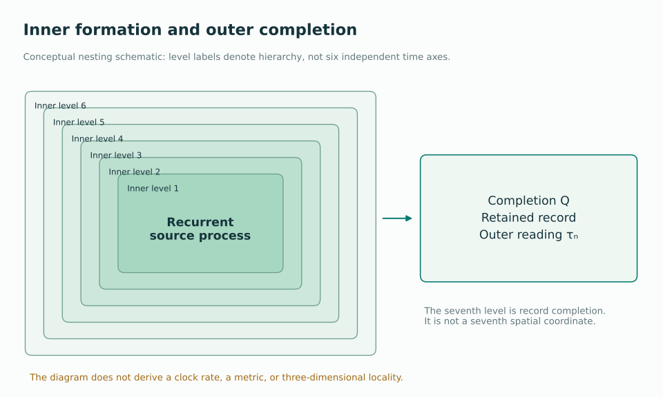
The familiar interpretation “two inner levels per spatial dimension” motivates a three-dimensional reading. Counting levels alone does not establish independent directions, local neighborhoods or a universal clock ratio. A physical update must produce those quantities, with each measurement independently defined. The constants program does not assume that dimension D automatically equals a physical clock ratio.
3 · What counts as an observable record?
Let histories act on underlying states x. Let Q be a completion map and O a family of tests on completed records. Declare two states equivalent if every admissible future history makes them indistinguishable by those tests:
This gives a future-stable observable quotient. It is a precise expression of the distinction between hidden formation and retained observation. However, Q, the test family and the dynamics are substantive physical choices. Different tests may produce different quotients. Geometry is not fixed by writing the equivalence relation alone.
4 · A conditional route to local rank three
The quaternionic construction supplies a useful mathematical example. A positive multiplicative norm, finite dimensionality, associativity and noncommuting phase directions select ℍ. Records that ignore its scalar center and transform covariantly under all connected inner automorphisms have the full rank-three vector readout W ≅ Im ℍ. Quaternionic conjugation supplies its ordinary rotational action.
Each condition has a role: associativity removes nonassociative alternatives; positivity removes split norm degeneracy; noncommutation excludes one complex slice. The second incompatible phase and record covariance still require dynamical explanations. A local vector module becomes physical space only after transport, compatibility of neighboring records, locality and a continuum or effective metric are established.
5 · Phase is not the same as split-complex time notation
A real skew-adjoint flow can, on its nonzero-frequency sector and with the proper domain conditions, yield a polar phase operator J with J² = −I. That is the ordinary complex structure used for U(1) phase. A split-complex unit j² = +1 is a different algebraic object. This explorer does not infer one from the other, or identify a hyperbolic boost with an ordinary quarter-turn rotation.
6 · One dictionary connects the sectors
| Quantity | Role in the construction | What remains to fix |
|---|---|---|
| a [J s] | Action per phase radian | Physical phase matching and standards |
| ℓ* [m], τ* [s] | Readout length and completion interval | Independent rods and clocks |
| υ | c = υℓ*/τ* | Common propagation law and Lorentz limit |
| K | Quadratic phase response | Physical gauge and charge matching |
| εₑ, εₚ | Dimensionless particle gaps | Electron and baryon sector dynamics |
| κ, r | Curvature and absolute vacuum coefficients | Metric response, normalization and stability |
gₑ = εₑ²/(16πκυ²), λₑ = rυ²/(2κεₑ²),
gₑλₑ = r/(32πκ²).
These are conditional identities with fixed conventions and a common scale. The electron and proton gaps must share a vacuum and clock. Dimensionless relationships are the strongest targets because arbitrary conversion units cancel. The dictionary organizes a unified problem; it does not calculate its own inputs.
7 · How to read claims in this website
| Label | Meaning | Example |
|---|---|---|
| Postulate | An organizing starting principle | Completed records come after inner generation |
| Extra assumption | A selected mathematical or physical rule | Use the free symmetric receiver |
| Model result | A consequence within those rules | dim Sym²ℂ⁴ = 10 |
| Open interface | A physical identification still needed | Match determinant phase to electromagnetism |
| Target reused | A measured value fixes an input that returns it | Fit κ from G, then calculate G |
8 · Suggested reading route
- α: see how local rank, quadratic closure and branches lead to 137, then why a response calculation is still required.
- ℏ: distinguish a theorem about phase from selection of a dimensional scale.
- Electron mass and mass ratio: follow excitation gaps and common-scale cancellation.
- G and Λ: inspect the two coefficients of one geometric action.
- Compare: change a shared parameter and inspect which sectors depend on it.
Source basis: C · §§2–5 and §14; pp. 4–8, 22–23. These explanations summarize the stated models; they do not add a new physical selection theorem.
Source basis: Q · §§1, 4–9; pp. 1–2, 9–19. These explanations summarize the stated models; they do not add a new physical selection theorem.