Fine-structure constant

SIMPLIFIED DERIVATION & CONCEPTUAL CONNECTION

How could a dimensionless interaction strength emerge from temporal completion?

The structural construction gives an exact rank 137 and a normalized determinant phase 1/137. A separate completion model calculates a response stiffness. Connecting either result to physical electromagnetic coupling requires a charge convention, a gauge action and a matching prescription.

Read the common SMM/DTT foundations and notation →
Jump to the live workbench ↓

The SMM/DTT connection

SMM assigns generative priority to one source; DTT distinguishes its inner formation processes from the outer records we observe. For electromagnetism, the useful question is how a small phase mismatch changes the weight of a completed record. The curvature of that response is a candidate stiffness. It is more informative than a raw count because it depends on how hidden histories are actually composed and eliminated.

Route A · The structural 137, step by step

Obtain a conditional three-component readout

Assume a finite-dimensional associative real carrier with a positive multiplicative quadratic norm and two noncommuting complex phases. These hypotheses select the quaternion algebra ℍ. A nonzero record family that ignores the scalar center and is covariant under all connected inner reorientations then spans the full imaginary-quaternion vector module:

W ≅ ℍ / ℝ1 ≅ Im ℍ ≅ ℝ³.

This is a real vector-space quotient. The algebraic and record assumptions are essential. A local rank-three readout still needs transport, gluing and locality to become physical space.

Retain symmetric pair data

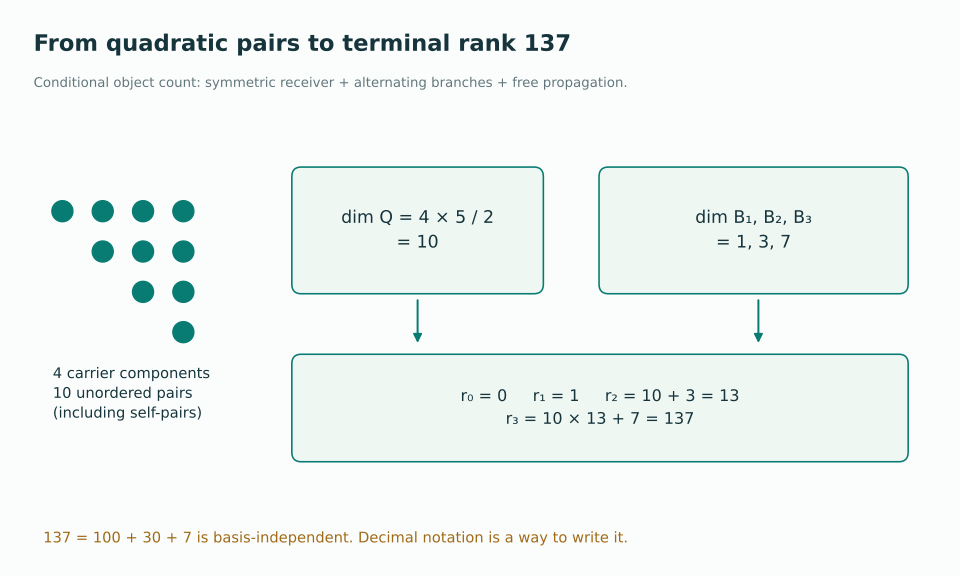
Adjoin the scalar component and complexify: U = ℂ ⊗ℝ (ℝ ⊕ W) has complex dimension four. If completion retains all symmetric quadratic pair data with no further relations, its receiver is Q = Sym²ℂ U. Four self-pairs and six distinct mixed pairs give:

dimℂ Q = 4(4 + 1)/2 = 10.

For a flag W₀ ⊂ W₁ ⊂ W₂ ⊂ W₃, the corresponding quadratic dimensions are 1, 3, 6, 10. Their successive increments are 1, 2, 3, 4. Thus ten is the dimension of one specified quadratic object. Selecting this free receiver is an additional construction rule.

Count the nonempty alternating branches

At depth d, take a d-dimensional complex innovation space I_d. Its free exterior algebra retains alternating combinations. Removing the empty combination gives:

B_d = Λ^≥1I_d, dim B_d = Σ_k=1^d C(d,k) = 2^d − 1.

The branch counts at depths 0, 1, 2, 3 are 0, 1, 3, 7. The alternating law and the decision to retain the free object must be justified by a future microscopic theory.

Propagate old sectors and add new branches

The proposed free reconstruction carries each earlier sector through Q, then adds the new branch sector. Tensor products multiply dimensions; direct sums add them:

R₀ = 0, R_d = (Q ⊗ R_d−1) ⊕ B_d.
r₀ = 0, r₁ = 1, r₂ = 10 × 1 + 3 = 13,
r₃ = 10 × 13 + 7 = 100 + 30 + 7 = 137.

This calculation is exact within the stated construction. It does not explain the historical adoption of decimal notation: the same dimension is 137 in base ten and 10001001 in base two.

Ten symmetric pair components and the rank sequence zero, one, thirteen, one hundred thirty-seven — Figure α1. The rank follows from the specified symmetric, exterior and propagation rules. The image does not identify these components as elementary particles. Download SVG

Extract a structural phase

A scalar phase z acting on an n-dimensional complex space has determinant zⁿ. Requiring determinant one restricts z to the n-th roots of unity. For R₃:

det(zI₁₃₇) = z¹³⁷ = 1,
z = exp(2πik/137), ϑ₁₃₇ = (least positive phase)/(2π) = 1/137.

The phase ϑ₁₃₇ may be proposed as a candidate α₀ only after a physical identification. A determinant phase, a Hopf Chern degree and an electromagnetic interaction strength are different quantities.

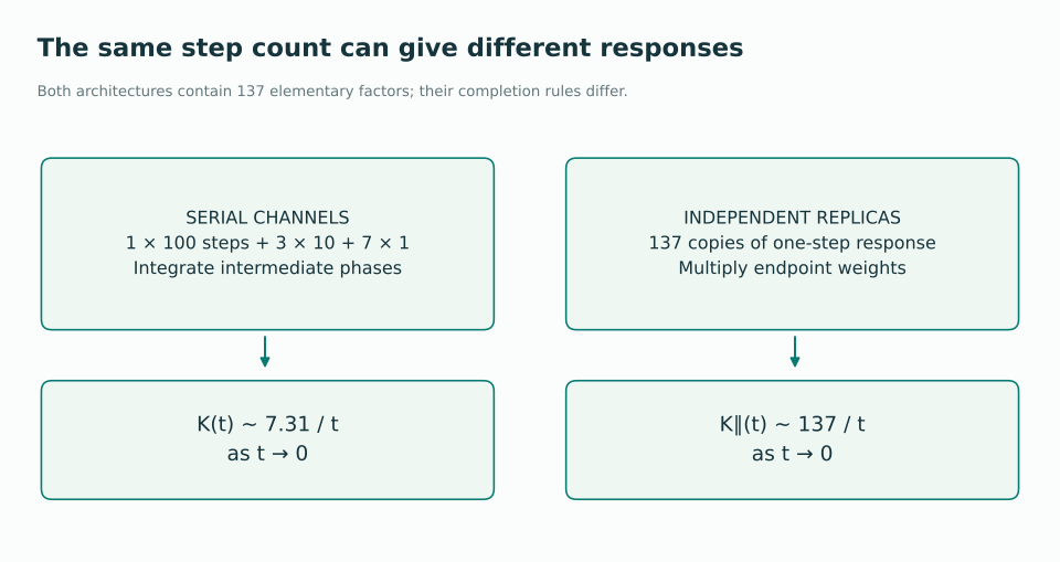
Route B · Calculate the retained response

Choose the circle heat kernel H_s(F) = Σ_n∈ℤ exp(−sn²/2) exp(inF). Convolution of L identical steps gives H_Lt; independent channels conditioned on the same endpoint multiply. For B = (1,3,7) channels with lengths L = (100,10,1):

W_t(F) = ∏_d=1³ [H_Ldt(F)/H_Ldt(0)]^Bd,
V_t(F) = −log W_t(F), K(t) = V″_t(0) = Σ_dB_dm₂(L_dt).

Here m₂(s) is the second moment of the normalized discrete Gaussian proportional to exp(−sn²/2). It is a computable response of the chosen completion rule. If this response yields a Maxwell term K F²/4, with electron charge convention qₑ = 1 and the required continuum matching, canonical normalization gives α⁻¹ = 4πK. The existence and normalization of that physical limit remain to be derived.

Serial completion and independent replica architectures have the same step count but different stiffness — Figure α2. At small t, serial completion has K ~ 7.31/t while 137 replicas have K ~ 137/t. The number of factors alone does not select coupling strength. Download SVG

Why α appears as a speed ratio in hydrogen

In the nonrelativistic Coulomb model with a fixed proton, E₁ = −mₑc²α²/2 and the virial theorem gives ⟨T⟩ = −E₁ = mₑ⟨v²⟩/2. Therefore v_rms/c = α in the ground state. This is a root-mean-square quantum speed, not a literal circular trajectory. For a finite proton mass, v_e,rms/c = (m_red/mₑ)α in the center-of-mass frame, with m_red = mₑmₚ/(mₑ + mₚ). Since α already enters the Coulomb Hamiltonian, this relation interprets the coupling; it does not independently calculate its value. Standard hydrogen reference →

What would complete the physical derivation?

Derive the receiver and completion rules from source dynamics; identify the physical electron representation; calculate a gauge-invariant transverse response with a fixed normalization; control its continuum limit and low-energy matching. The residual 137.035999177 − 137 = 0.035999177 must then be calculated rather than assigned a name such as holonomy correction.

Try the workbench

Compare the structural and response routes. In the response route, change t and switch the composition architecture. Activate “Fit t” to see the target-reuse cycle. The summary figures are fixed illustrations; the workbench and comparison page show your current settings.

Source basis: Q · §§4–9; pp. 9–19. These explanations summarize the stated models; they do not add a new physical selection theorem.

Source basis: C · §§6–10; pp. 8–18. These explanations summarize the stated models; they do not add a new physical selection theorem.

Explore α.