The temporal origin of distance: reconstructing a metric from records

01Conceptual and physical setting

A dimension can count independent coordinates, the growth of accessible states, or the response of a diffusion probe. Those counts agree for ordinary smooth Euclidean space, but they need not agree for a discrete network or a scale-dependent geometry. A three-component observable therefore establishes less than a three-dimensional physical space: the latter also requires points or records, overlap relations, a metric, and a controlled regime in which nearby records behave continuously.

This distinction makes dimensional emergence a precise question. If the source produces records with labels in a three-dimensional vector space, their actual arrangement might still be a line, a disconnected set, or a dense cloud with nonlocal transport. The physical dimension concerns how those records can be compared and traversed. A convincing construction ties the algebraic number of directions to volume growth and propagation using the same dynamics. ^{[4] [3]}

02Why retained relations matter

The Single Monad is nonspatial, so its alleged unity cannot be represented as a point that sends ordinary signals from a hidden location. In DTT, locality would belong to the relations among completed records. The six inner levels could produce and retain a neighborhood structure; outer time would order observable influence through that structure.

A single controller is not enough to explain locality if it is allowed to update any record pair independently. A stronger rule lets the same retained relations restrict both record formation and later transport. Then memory is physically important: it preserves which comparisons count as nearby, rather than being an inert log appended after spatial interactions have already been assumed.

03Worked graph metric

Take four records A,B,C,D with edges A–B, B–C and C–D, each assigned length a. The shortest-path distances are d(A,B)=a, d(A,C)=2a and d(A,D)=3a. This is a legitimate metric because path concatenation gives the triangle inequality.

Now add a direct A–D edge of length a. The graph distance d(A,D) becomes a, even if a drawing still places D far from A. The physical geometry depends on the actual comparison and transport relations, not on where labels are displayed. A DTT source must therefore generate the edge data and explain why the measured metric agrees with the intended spatial readout. The example also shows why a finite propagation bound on graph edges cannot by itself establish locality in an independently drawn geometry.

04A two-record spectral distance

A simple spectral example makes the operator normalization visible. Let an algebra of diagonal two-by-two matrices act on C², with f=diag(f1,f2), and take D=[[0,m],[m,0]] for real m≠0. Then the norm of [D,f] is |m| |f1−f2|. The distance defined as the supremum of |f1−f2| under the constraint ‖[D,f]‖≤1 is therefore 1/|m|.

The operator encodes a distance, but its scale is not generated by the distance formula. Doubling m halves the distance. A source theory must select m or relate it to an independently generated clock and energy scale. This small calculation is useful because it distinguishes a valid reconstruction interface from a claim that every spectral triple automatically explains geometry. ^[1]

05The source-selection problem

SMM/DTT aims to derive the relational data from one nonspatial source. Six nested inner levels can organize the production of compatible comparisons, while outer completion retains the graph or operator accessible to observers. The key advance would be a rule that fixes adjacency and weights rather than choosing them independently to obtain the desired geometry.

A source can produce many records without producing a useful metric. Records may be disconnected, have arbitrary long links, or carry incompatible local distance assignments. A completion condition can reject such configurations, but its success probability and resource cost matter. Otherwise the model may simply postselect a rare spatial sector from an unrestricted state space.

The positive target is an autonomous law that generates and stabilizes a metric-compatible neighborhood structure. A separate propagation calculation can then test whether the same structure governs influence. If both follow from one retained-memory mechanism, the theory explains more than a graph chosen by hand. ^{[2] [3]}

06A transport check after distance has been reconstructed

On a chain with nearest-neighbor updates, suppose a disturbance can cross at most one edge of length a during each completed interval δτ. A record N edges away cannot respond before Nδτ, giving an exact circuit cone with v=a/δτ. This uses a bounded-depth update with strictly local gates.

Continuous-time Hamiltonians generally give a different result: a Lieb–Robinson estimate bounds a distant commutator by a constant times exp[−μ(d−vt)]. The tail is small rather than exactly zero outside the effective cone. If d−vt=10/μ, the exponential factor is about 4.54×10⁻⁵. Neither result determines a physical speed until the edge length and the clock interval are independently identified. Nor does either prove that the source generated the chain. ^{[2] [3]}

07Distance is not dimension

A graph can have a well-defined metric while its large-scale dimension differs from the number of entries in its local record vector. Spectral dimension can also depend on the diffusion clock. A strong source reconstruction therefore compares graph distance, volume growth, spectral behavior and material transport as independent outputs. Their agreement would turn rank-three algebraic readout into evidence for an actual three-dimensional geometry in a specified regime.

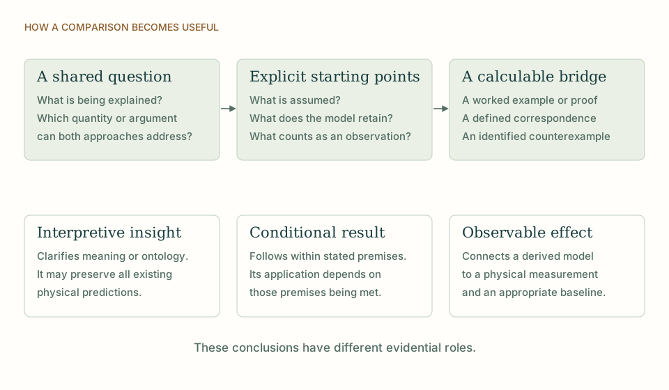
THE SAME QUESTION, DIFFERENT STARTING POINTS

The comparison at a glance

Continue on SMONAD

• Why spectral dimension does not determine distance →

  Develops the source construction or operational distinction used in this comparison.

• Graph distance from a normalized spectral block →

  Develops the source construction or operational distinction used in this comparison.

• Generating a neighborhood and preserving local transport →

  Develops the source construction or operational distinction used in this comparison.