Gravitational waves and temporal geometry: SMM/DTT and Causal dynamical triangulations
What would a temporal origin of geometry imply for the speed, polarization and phase evolution of gravitational waves? This article compares the source-based construction with Causal dynamical triangulations, identifies their strongest point of contact, and works through a concrete example that separates a valid mathematical result from the further physical relation needed to explain observations.
Gravitational waves test dynamics directly: a theory must describe their production, propagation and detection through material instruments. In general relativity their weak-field vacuum limit contains two transverse tensor polarizations propagating on the metric null cone. Modified gravity can change that pattern, but a microscopic theory need not produce any observable deviation at accessible frequencies.
A temporal interpretation of curvature becomes predictive only after its effective wave operator is known. Claims of dispersion, echoes or additional polarizations require a particular mechanism and boundary conditions. A finite inner update frequency alone does not determine whether a gravitational wave is dispersive; it may disappear entirely from the long-wavelength limit or enter only through highly suppressed operators. [1][2][3]
02The SMM/DTT contribution
SMM/DTT seeks to interpret geometry as the organization of completed records. A gravitational wave could then be a propagating collective change in relational timing and distance rather than a deformation of a pre-existing substance. This can be a useful microscopic picture if the same source update also governs how mirrors, atoms and clocks respond.
The six nested inner levels should be understood as the generative organization supporting this effective response. They do not imply six gravitational-wave polarizations. Observable polarizations follow from the constraints and physical degrees of freedom of the effective field equations. A clear derivation could recover the standard two modes and then identify a restricted residual correction whose coefficient is fixed by the temporal dynamics.
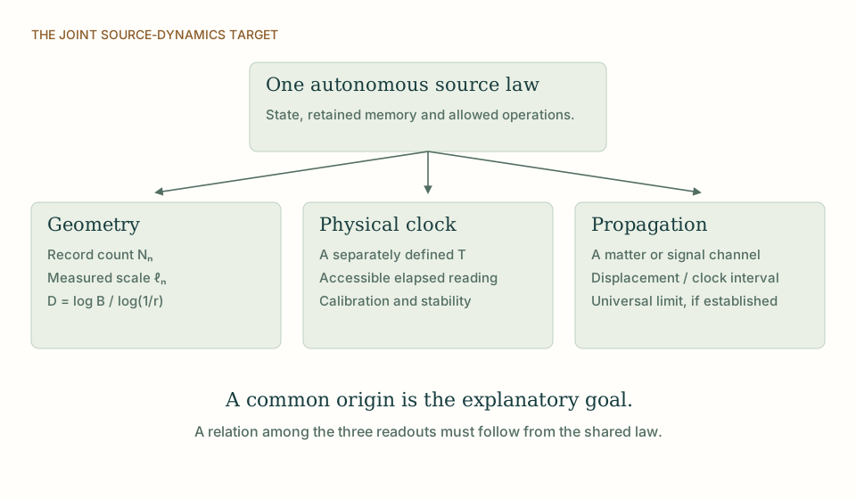
Geometry, clocks and propagation as independent readouts. A single source model should explain the relation between separately defined measurements. Sharing a diagram does not impose that relation. View full size ↗
03How Causal dynamical triangulations frames the problem
Causal dynamical triangulations defines a sum over discretized geometries with a specified causal organization and action. Macroscopic behavior is studied through ensembles and scaling, rather than by treating one fixed triangulation as the final spacetime. Diffusion-based dimension is one useful probe of the generated ensemble. Its numerical behavior is a result inside the model.
The comparison with DTT concerns how a regulated construction produces an extended geometry with stable large-scale observables. A nested inner process is not a triangulation time coordinate, and a computational update used to sample an ensemble is not an observer's clock. Distinguishing these roles is essential when interpreting emergent temporal and spatial behavior. [4]
04Where the mechanisms agree and differ
CDT investigates a gravitational ensemble, but deriving an observed gravitational-wave signal requires identifying perturbations with physical tensor modes and coupling them to a source and detector. A macroscopic geometric phase or a diffusion dimension alone is insufficient. DTT similarly needs to connect completed record fluctuations to a dynamical metric observable.
The comparison is useful because it separates Euclidean or statistical diagnostics from real-time propagation. A return-probability calculation can reveal effective dimension without determining the speed of a wave packet. The six nested inner levels may affect both diagnostics through the source law, but their equality is a result to establish, not a definition. A productive DTT construction would derive the quadratic effective action for metric perturbations and show how its time variable is read by material clocks. The multimessenger estimate below supplies a benchmark only after that operational identification. It cannot be applied directly to sampling time in a simulation or to an arbitrary source iteration. This is a realistic path from a discrete geometric model to phenomenology: first derive the physical propagator, then compare its observable phase and polarization with the established tensor-wave limit. [4]
05Worked example: assumptions, calculation and result
For a simple nondispersive propagation comparison, take a source distance of 40 megaparsecs and an arrival-time difference of 1.7 s. Since 1 Mpc≈3.086×10²² m, the travel time is approximately 4.12×10¹⁵ s. Dividing gives |Δv|/c≈4.1×10⁻¹⁶ if the entire delay is attributed to propagation.
This arithmetic is only an illustrative inference. Electromagnetic and gravitational signals can leave the source at different times, and cosmological propagation requires a more careful treatment. The published GW170817 analysis incorporates astrophysical assumptions in its bounds. A DTT wave-speed claim must specify those same assumptions and cannot equate the observed arrival delay directly with an intrinsic inner-time lag. [1][2][3]
Δv/c≈Δt/(D/c). For D=40 Mpc and Δt=1.7 s, the propagation-only estimate is 4.1×10⁻¹⁶.
D is the source distance in this approximation; the sign and magnitude of an intrinsic emission lag are separate inputs.
06An independent operational check
A proposed dispersion relation can be tested internally before fitting data. Its frequency must remain real for the intended wave numbers, its energy should be bounded in the physical sector, and its group velocity should be interpreted separately from its phase velocity. A higher-derivative term may introduce an extra mode or an instability if treated beyond the effective theory's domain. The source programme is strongest when it states that domain and derives the coefficient there. These checks connect microscopic temporal structure to a viable propagating signal; they also prevent an arbitrary frequency-dependent delay from being mistaken for a complete gravitational-wave theory.
07What follows from the comparison
The strongest experimental target is a correlated signature: the same effective coefficient might affect wave phase, matter clocks or another transport probe. Agreement among these effects would be more informative than fitting a single unusual signal. Until a source-derived coefficient exists, gravitational-wave observations provide consistency requirements and a way to translate possible models into bounds, rather than existing confirmation of temporal geometry.
THE SAME QUESTION, DIFFERENT STARTING POINTS
The comparison at a glance
Question
SMM/DTT
Causal dynamical triangulations
Starting physical structure
One nonspatial source; six nested inner functional levels produce records accessible through outer completion.
An ensemble of causally organized piecewise-flat geometries.
The central mechanism in this topic
Metric fluctuation amplitudes need an operational clock and detector coupling.
Geometric ensembles must yield physical real-time perturbations before wave predictions follow.
How the claim is made operational
A source-to-record map must define geometry, material response and physical clocks with shared inputs.
Path-sum weights, numerical observables and refinement toward a continuum regime.
Meaning of agreement
Agreement is a compatibility result; a source-selected relation or fixed residual would add explanatory content.
The stated framework provides a benchmark within its own assumptions and established domain.
KEEP THE CONNECTION
Key ideas
Diffusion data and wave propagation test different aspects of an emergent geometry.
The worked example establishes only the result stated under its explicit assumptions.
Six nested inner levels describe one generative organization; outer time orders accessible completion.
Develops the source construction or operational distinction used in this comparison.
Sources and further reading
References support the comparator and the specific mathematical or interpretive claims indicated. SMM/DTT connections are developed in the analysis above.