Rapid hidden relaxation yields a local effective response when observable motion remains slow. Its positive semidefinite metric, approximation error, and uncoupled directions follow from explicit operator and timescale assumptions.
A hidden response can sometimes be replaced by an almost instantaneous effect, but only when its relaxation is fast relative to the visible motion. The leading reduction produces a local matrix response with controlled corrections. This article identifies the symmetry, timescale, and coupling conditions needed before SMM/DTT can interpret that local equation as an effective outer description.
02The required separation of scales
A local reduced law becomes plausible when hidden modes relax much faster than q changes. If λ_min is the smallest relevant relaxation rate and τ_q the observable evolution timescale, require λ_minτ_q≫1 and observe after the initial transient. One must also control the size and variation of the coupling and gradient. A large symbol Λ in an equation is not enough if the observable itself develops comparably rapid motion or if a hidden nearly stationary mode remains coupled.
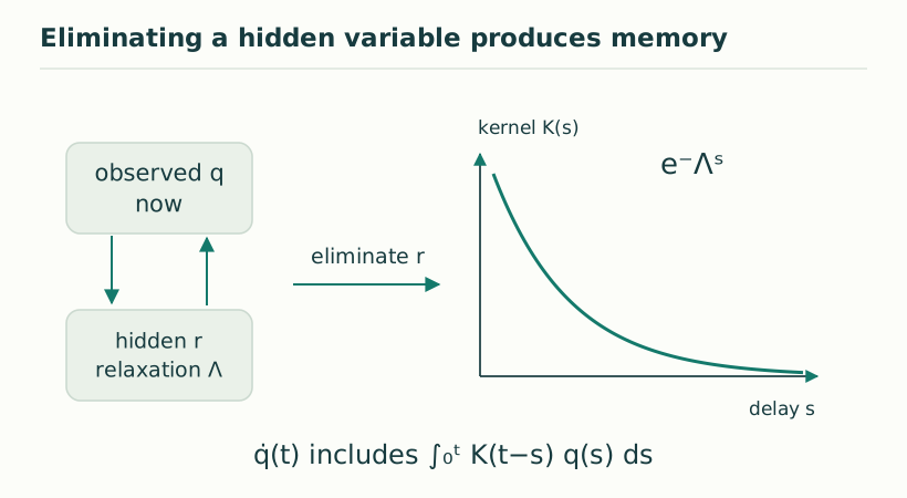
Figure 1. Eliminating a hidden variable produces memory. For a linear relaxing hidden sector, substitution produces a Volterra memory term. An exponentially decaying kernel is the simplest example; its fast limit can yield local effective dissipation under additional assumptions. View full size ↗
03The adiabatic elimination
Expand ∇Ψ(q(t−u)) around its current value inside the exponentially weighted memory integral. The leading integral is ∫₀∞e^(−Λu)du=Λ⁻¹ on the stable hidden sector. This gives r≈−Λ⁻¹Kᵀ∇Ψ and q̇≈F(q)−M∇Ψ, with M=KΛ⁻¹Kᵀ. For symmetric positive-definite Λ, M is positive semidefinite because vᵀMv=(Kᵀv)ᵀΛ⁻¹(Kᵀv)≥0. Mere stability without the relevant symmetry or dissipative structure requires a more careful argument.
M=KΛ⁻¹Kᵀ
vᵀMv≥0 when Λ=Λᵀ>0
04An explicit error scale
For the scalar convolution I(t)=∫₀ᵗe^(−λu)q(t−u)du, its leading approximation is q(t)/λ. After the initial transient, the first correction is −q̇(t)/λ². Thus the relative correction is controlled by approximately 1/(λτ_q), provided q is not crossing a zero that makes a relative estimate meaningless. Absolute derivative bounds are safer near such zeros. This small calculation explains why fast-response laws fail during sharp pulses even when they work well for slow evolution.
I(t)≈q(t)/λ−q̇(t)/λ²+⋯
05What the approximation can and cannot establish
The effective matrix M tells which observable directions are dissipative and which lie in its kernel. It does not select the structural functional, prove thermal equilibrium or determine a physical clock. Comparing the exact memory model with its local limit over several driving frequencies provides a clear validation of the approximation. In SMM/DTT this is the appropriate meaning of an outer effective law: it summarizes a declared generative response in a controlled regime, while retaining an explicit account of the information and timescales that were removed.
06A kernel direction can survive completion
If Kᵀv=0, then vᵀMv=0 even when every hidden mode relaxes rapidly. The observable direction v simply does not couple to that hidden channel. For example K=(1,0)ᵀ with scalar Λ=λ gives M=diag(1/λ,0). One coordinate is damped and the other is untouched by this mechanism. A unique equilibrium therefore needs more than fast relaxation: it requires appropriate coupling rank and a structural functional with suitable minima, together with control of reversible motion. This is an important model-building check when a completion process is claimed to erase all generative distinctions or produce one universal arrow.
07Interpretation of an irreversible reduced law
A reduced equation can lose predictive information because several larger states share one observed state. That does not make projection alone a universal source of thermodynamic entropy. Positive hidden relaxation, a chosen initial condition or reservoir, and a condition on the reversible flow do essential work in this model. The structural functional Ψ is not automatically Boltzmann, Gibbs or von Neumann entropy. Connecting its decay to a laboratory second law requires an operational coarse-graining, thermodynamic variables and calibrated coefficients. This qualification preserves the useful mechanism while preventing a model-level monotonicity theorem from being mistaken for an unconditional derivation of time’s arrow.
A finite closed Hamiltonian system preserves information globally and can display recurrences. Replacing some of its degrees of freedom by a permanently relaxing operator requires a specified approximation, reservoir or limiting regime. The exactness claimed for hidden-variable elimination is exactness relative to the supplied coupled equations, including their positive relaxation operator. It is not an independent proof that those equations follow from a conservative temporal action. A source-based derivation should track where the discarded information resides and over which interval the reduced dissipative description remains accurate.
KEEP THE CONNECTION
Key ideas
Fast response requires a quantified separation of timescales.
Derivative corrections identify when the local approximation fails.
Scope of the argument. Controlled leading-order approximation under stable fast relaxation; positivity needs the stated operator assumptions.
Sources & further reading
dual_time_entropy_v4.pdf — working draftpp. 16–19 and 22–23, §§6.6–6.11
Source editions and catalogue entries
Working manuscript
A Dual-Time Gauge Model for Projection-Induced Memory and Irreversibility
Working manuscript. Article-level references identify the consulted sections and the scope of the interpretation. No public URL was supplied for this exact manuscript version.