What is retained by a holonomy?

A closed route can remember more than its endpoint

Transport a retained orientation or phase through a sequence of local frames and return to the starting record. The endpoint can be the same while the transported carrier has changed. Holonomy is the resulting transformation around that closed route. It offers SMM/DTT a precise language for information retained through generative transport, provided the carrier, links and completion experiment are explicitly defined.

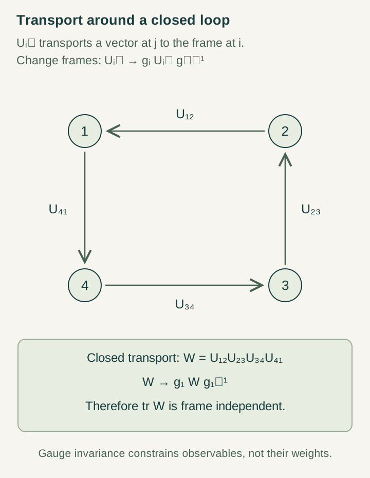
The relevant memory is relational. A link matrix depends on the chosen frames at its endpoints; a physically meaningful loop comparison must remove that arbitrary choice. The holonomy guide develops this distinction, and the interactive loop demonstration lets readers change frames while checking the invariant result.

The frame changes cancel around a finite loop

Take three records labelled zero, one and two. Let U₁ transport from zero to one, U₂ from one to two, and U₃ from two back to zero. The complete transport is W=U₃U₂U₁. Under local frame changes g₀, g₁ and g₂, the links become g₁U₁g₀⁻¹, g₂U₂g₁⁻¹ and g₀U₃g₂⁻¹.

The matrices at the intermediate records cancel. The loop changes by conjugation at the base point, so its eigenvalues and traces in a declared representation are unchanged. For abelian U(1) links, conjugation has no effect and W itself is invariant.

As a numerical example, assign link phases π/6, π/3 and π/2. Their sum is π and W=−1. Rephasing a record adds a phase to one adjacent link and subtracts it from the other, leaving the sum unchanged modulo 2π. This is an exact finite identity. Interpreting the phases as electromagnetic transport requires a calibrated connection to a physical field and a charged carrier.

A holonomy needs a specified readout

A transformation written in the model is not automatically accessible to an observer. One experiment sends a coherent amplitude along the loop and compares it with an untransported reference path. If the carrier begins in ψ, the positive recombination port has probability ‖(I+W)ψ‖²/4. For a scalar W=e^iθ, this is [1+cosθ]/2.

A different experiment uses a carrier and a co-located dual prepared in the normalized neutral state s=(1/√d)Σₐ|a⟩|ā⟩. Sending only the carrier around the loop gives return amplitude ⟨s|(W⊗I)|s⟩=Tr(W)/d. A sharp neutral-return test has probability |Tr(W)/d|². This is a particular character-sensitive readout, not a complete measurement of every matrix entry.

The Aharonov–Bohm paper is an original physical reference for phase-sensitive effects associated with electromagnetic potentials. Wilson's lattice-gauge construction supplies the broader loop-variable setting. The finite calculations here are a way of stating exactly what an analogous source experiment would retain.

Different retained probes can miss different structure

Suppose W=diag(e^iθ,e^−iθ) in the defining two-dimensional representation of SU(2). Its normalized trace is cosθ, and the neutral-return probability is cos²θ. That probability alone cannot distinguish every θ that has a different trace, because squaring removes its sign. A phase-sensitive reference experiment can retain information that a probability-only singlet return discards.

The central transformations I and −I give an even simpler comparison. Acting on an isolated carrier density matrix, both induce the same channel ρ↦ρ. Acting on only one branch of a path interferometer, they produce opposite relative phases. In the adjoint representation of SU(2), both central elements act identically. Observability therefore depends on the representation, reference and available controls.

There can also be an entirely inaccessible sector. Let a source transport be W⊕V, but suppose every preparation lies in the first block, every evolution preserves that block and every completed test acts only there. Changing V changes no prediction for that operational domain. The inaccessible-holonomy article explains why a claim about hidden curvature needs a reachable preparation and a distinguishing continuation.

Noncommuting routes add another retained distinction. Choose SU(2) transports U=−iX and V=−iZ. Their group commutator UVU†V† equals −I, whereas commuting transports give I. Both results leave an isolated carrier density matrix unchanged, but a coherent reference path distinguishes them through a relative minus sign. In this example the positive recombination probability is zero for the commutator loop and one for the identity loop.

A sequence of local direction displays can therefore miss information that a phase-bearing closed-history experiment retains. Conversely, a neutral-return probability by itself is one for both I and −I, so that test misses the distinction too. The example is a useful design tool: choose the retained record and reference according to the invariant one intends to measure, then verify the result under local changes of frame.

A small-loop response does not determine the full dynamics

A measured energy response near one holonomy can be summarized by a Hessian, the matrix of second derivatives. That local quadratic information is useful for stiffness and linear response. It does not determine the response at finite transport angles or identify every hidden sector contributing to the energy.

For a one-parameter example, compare E₁(θ)=a(1−cosθ) with E₂(θ)=(a−4b)(1−cosθ)+b(1−cos2θ), where a>0 and 0<b<a/4. Both are nonnegative and satisfy E₁″(0)=E₂″(0)=a. At θ=π, however, E₁=2a while E₂=2a−8b. Identical quadratic response leaves a finite-angle difference.

Consequently, obtaining a holonomy Hessian or a representation index does not alone determine an entire gauge theory, its charge normalization, particle spectrum or interaction law. The response-Hessian discussion identifies these separate inputs. A source construction can strengthen its result by deriving linked higher-order responses from the same parameters.

What a source-based holonomy result should deliver

Specify a finite network of completed records, one carrier representation and allowed source transports. Define the local frame equivalence and prove it survives the work update. Then state how an observer prepares a reference, traverses a loop and reads a completion result. The retained record should predict a later experiment without requiring hidden information that the source has discarded.

A useful challenge is to choose two transports that agree on the first proposed readout and construct a second allowed test that separates them. If no such test exists under all admitted continuations, characterize the observable equivalence class instead of assigning empirical significance to the hidden difference. For a response model, calculate both the local curvature and one finite-loop observable with the same calibrated couplings.

This makes holonomy an effective meeting point for geometry, quantum theory and research methodology. It records how a carrier returns, explains which changes are frame conventions, and demands a physical experiment for every claimed retained distinction.

Continue reading

• Holonomy: what a closed path remembers →
• Change local frames without changing a loop holonomy →
• A singlet-bound loop with an exact energy response →
• What the holonomy Hessian does and does not contain →
• Invisible holonomy in inaccessible sectors →

Read this discussion as part of a path

• Phase, gauge structure and field theory →