Does a finite gap solve the Yang–Mills problem?

A finite gap can be an important theorem

A source construction may yield an explicit Hamiltonian with a stable lowest state and a positive energy separation above it. Proving that separation, particularly under controlled perturbations, is useful mathematics. It can support a retained excitation, a reliable completion sector or a tractable gauge model.

The Yang–Mills existence and mass-gap problem asks for substantially more. The official Jaffe–Witten problem description concerns a nontrivial quantum Yang–Mills theory on four-dimensional spacetime for a compact simple gauge group, with the required field-theoretic properties and a positive gap. A result for a finite matrix, one compact circle or one selected charge sector has a different domain.

For SMM/DTT, a productive discussion should identify precisely which gap has been established and then ask how that result behaves when the regulator, volume and accessible sectors change. The site's discrete Yang–Mills reading guide is organized around that distinction.

A perturbatively stable finite example

Take H₀=diag(0,Δ,2Δ) with Δ>0. Its unique lowest state is separated from the next state by Δ. Add a self-adjoint perturbation V with operator norm at most ε. Each ordered eigenvalue changes by no more than ε: the Rayleigh quotient of any normalized vector changes by at most that amount, and the min–max characterization transfers the bound to eigenvalues.

The inequality is a complete and useful finite statement. It does not depend on a numerical diagonalization at one chosen parameter value. A source model can gain real strength by proving an analogous uniform estimate for its admitted finite perturbations.

What the estimate covers must remain explicit. The Hilbert space, all its sectors, the energy unit and the allowed perturbation norm were fixed. If refinement adds new states or rescales the Hamiltonian, one needs a new argument connecting those changes with the lower bound. A gap protected inside a fixed sector need not be the lowest excitation of the enlarged system.

A charged threshold can coexist with arbitrarily low neutral excitations

Suppose the retained charged model has its first excitation at Δ. Add an independent neutral two-level system with energies zero and ε. The total Hamiltonian is H_charged⊗I+I⊗diag(0,ε). Its lowest excitation lies at min(Δ,ε), even though the charged threshold remains exactly Δ.

Let ε decrease along a sequence of regulators. Every charged-sector calculation can remain unchanged while the full gap tends to zero. Calling the new sector neutral does not make it irrelevant: the physical question is whether it belongs to the gauge-invariant Hilbert space and can contribute to the theory's excitations or local observables.

The charged-threshold article develops this missing-sector issue. A proof must identify all physical sectors and explain why no omitted sequence carries vanishing excitation energy. Excluding a sector is legitimate only when a stated physical constraint, rather than the desired conclusion, removes it.

A simple lattice gap disappears as the box grows

Consider a periodic chain of N sites with lattice spacing a and discrete Laplacian −Δ_a. Let H=κ(−Δ_a), where κ sets the energy–length-squared unit. Its Fourier modes have energies E_k=(4κ/a²)sin²(πk/N). Removing the constant ground mode leaves a first excitation that is positive for every finite N.

At fixed spacing a, increasing the physical length L sends this gap to zero. Refining the lattice at fixed L instead leaves the positive limiting value 4π²κ/L², which is a box-size scale. Thus a sequence can have a positive gap at every finite step and still fail to produce a nonzero infinite-volume mass gap.

This example is a scalar lattice calculation, not Yang–Mills dynamics. Its role is logical: it demonstrates why positivity at each regulator does not imply a uniform physical lower bound. The same question must be asked of any compact inner-time spectrum or finite completed-record Hamiltonian.

What compact inner time actually supplies

On a circle of radius R, the operator −d²/ds² has eigenvalues n²/R². Restricting to nonconstant functions gives a positive spectral threshold 1/R². The result concerns that operator, that radius and that function space. Converting it into an energy gap needs a calibrated Hamiltonian, and converting it into a particle mass needs the relevant energy–momentum interpretation.

A Gauss-law constraint is a condition of gauge invariance on physical states. It cannot be assumed to remove every zero-frequency or neutral degree of freedom merely because that removal would produce a gap. The physical kernel should be derived from the actual constraint operators. The vacuum and the excitations above it must then be identified inside that physical space.

If R is a regulator, the bound must be tracked as the regulator changes. If R is proposed as a fixed physical source scale, the model must explain how its low-energy continuum limit retains that scale without simply inserting a mass term into the desired conclusion. Either possibility is a well-defined research programme when its assumptions are stated.

Which next theorem would move the construction forward?

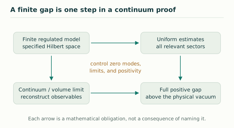
A useful staged programme begins by specifying an indexed family of gauge-invariant source Hamiltonians and a common physical calibration. Identify all neutral and charged sectors, then prove a lower bound uniform in the parameters that will be removed. Separately show convergence of the observables and correlation functions needed to define a nontrivial limiting field theory. A lower bound is meaningful only when the limit and its physical states are also controlled.

The field-theory task includes locality, covariance or their appropriate reconstruction conditions, positive probabilities and the short-distance behavior of the intended Yang–Mills model. A finite source can be a regulator or a useful model of one mechanism. Establishing which limiting theory it defines is a distinct result that cannot be inferred solely from the name assigned to its link variables.

Even a volume-independent bound does not identify the field theory by itself. Put one independent two-level system at each of N sites and use H_N=ΔΣⱼ|1⟩⟨1|ⱼ. The unique ground state has every site in zero, and the first excitation costs Δ for every N. This gives an exact uniform gap with no difficult spectral calculation. It supplies no interacting gauge transport or Yang–Mills correlation structure. A proposed source limit must establish the intended local observables and interactions as well as the energy bound; otherwise it might converge to a different, equally gapped theory.

For an immediate collaboration, choose one existing finite SMM/DTT gauge Hamiltonian and perform the missing-sector and scaling audit. Derive one uniform inequality, or construct a neutral or long-wavelength counterexample that invalidates a proposed bound. The remaining-gap guide and finite singlet-gap calculation provide concrete starting points. A precise partial theorem is valuable because it tells the next researcher exactly what remains to be proved.

Continue reading

• A discrete Yang–Mills proposal: which gap is being proved? →
• A protected gap in the finite singlet model →
• A charged threshold is not a full mass gap →
• The remaining gap-proof obligation →
• A singlet-bound loop with an exact energy response →

Read this discussion as part of a path

• Phase, gauge structure and field theory →