


The answer in brief
A causal cone restricts influence. A physical metric, universal matter coupling and a selected gravitational response law are additional results to derive.
Go to the research challengeA causal cone is a statement about allowed influence
A source construction may assign a completed displacement Δx and a completion delay Δτ to each allowed process. Suppose its path length obeys L≤vgΔu, its activity satisfies Δu≤DΔτ, and the spatial readout satisfies ‖Δx‖≤L. Combining these supplied inequalities gives ‖Δx‖≤vgDΔτ. This is an exact bound for the declared operations.
The resulting c*=vgD is a maximal allowed conversion under that interface. Establishing an attained propagation speed, a universal material clock and a three-dimensional Euclidean readout requires checking each corresponding construction. The published completion framework treats its cone in this conditional downstream role. A cone theorem is therefore a useful kinematic milestone with a definite domain, while a gravitational field equation remains a further target.
What does preserving a null cone leave undetermined?
In units c=1, the Minkowski quadratic form is −dt²+dx²+dy²+dz². Multiplication by any positive function Ω² leaves its null directions unchanged, because Ω²q(v)=0 exactly when q(v)=0. Thus a cone field does not select the local scale used by clocks and rulers.
For a stationary coordinate path, the metric η assigns proper duration ∫dt, while the conformally related metric Ω(t)²η assigns ∫Ω(t)dt. With Ω(t)=1+t on the interval 0≤t≤1, the durations are one and three halves. The null directions agree throughout. A physical clock comparison can distinguish the metric representatives, but the cone alone cannot.
This finite integral exposes why the conformal-calibration problem matters. One must define a matter clock or volume standard that selects a representative and prove that different calibrated devices agree on it. Naming one representative the physical metric does not provide the required clock mechanism.
What does an exact Lorentz transformation establish?
For β=3/5, the Lorentz factor is γ=5/4. The transformation t′=γ(t−βx), x′=γ(x−βt) sends the null displacement (t,x)=(1,1) to (1/2,1/2). It preserves the interval and this null direction exactly. This is the algebraic content illustrated in the Lorentz-transformation guide.
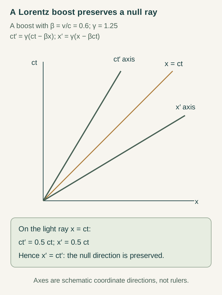
A source reconstruction must also identify which physical rods and clocks realize these coordinates and how transformations between their completed measurements arise. Even if that succeeds, it has not specified how matter changes the geometry. Flat-spacetime propagation and gravitational backreaction answer different questions.
Why a metric does not select its field equation
Suppose a smooth metric has already been obtained. One possible gravitational action is proportional to ∫√−g(R−2Λ), while a second adds β∫√−gR². The two actions use the same metric variable and can share a flat background, but varying them generally gives different dynamics. The coefficient β is new physical information.
The point does not depend on advanced curvature calculus. In a scalar analogy, the same configuration coordinate q can have potentials q²/2 or q²/2+βq⁴. Both identify the same variable and the same infinitesimal kinetic metric, yet their nonlinear forces are −q and −q−4βq³. Knowing the geometry of a configuration space does not determine the force law on it.
A gravity programme therefore needs a principle selecting its effective action or field equation, an identification of the matter stress tensor and a normalization of the response. A common limiting speed constrains the kinetic organization but cannot by itself fix G, Λ or every higher-curvature term.
What could a thermodynamic route contribute?
Jacobson’s Thermodynamics of Spacetime: The Einstein Equation of State derives the Einstein equation using a local horizon entropy–area relation, a heat–entropy balance and the accelerated-observer temperature. It demonstrates a concrete route from additional physical principles to a gravitational equation; the causal structure participates in a larger argument.
For SMM/DTT, this suggests a focused question: can the source define the relevant horizon records, their entropy and the energy crossing the horizon with one normalization? A count of available records must first be tied to an entropy functional and a physical area. A completion delay must be tied to a temperature or energy scale through an independently specified measurement. Importing those relations as assumptions can produce a conditional reconstruction; deriving them from the source would close a new interface.
The matter side is part of the derivation
A geometric field equation needs a source whose energy and momentum are independently defined. In a variational model, the matter stress tensor follows by varying the matter action with respect to the metric. Using that definition inside an assumed Einstein equation is standard model construction. A source derivation must explain why the same geometry controls both the matter kinetic term and its gravitational response.
Conservation also requires a declared total system. A visible record can exchange energy with hidden source memory, so its own energy need not be conserved. The complete source may conserve a total charge while the projected matter stress obeys an exchange equation. Before comparing with a covariantly conserved gravitational source, identify the hidden contribution and the regime in which it is negligible or included. This is a practical reason to connect the gravity problem to retained memory.
A maximum allowed speed need not be the observed propagation speed
A completed step may satisfy |Δx|≤Δt in calibrated units while the only propagating excitation available in the model moves by Δx=Δt/2. The unit cone is a valid bound, but no admitted excitation saturates it. Introducing a second species with Δx=Δt/3 preserves that bound and creates another propagation speed.
A common-speed theorem must therefore identify the characteristic or group-velocity limit of the actual matter and signal dynamics. It should prove saturation or a controlled limiting approach, and explain why all relevant species share the result. This is a separate task from showing that every completed motion stays inside a chosen cone.
The distinction is particularly useful in finite source models, where a broad resource bound may be easier to prove than a sharp propagation law. Reporting both tells readers exactly which kinematic freedom remains before any gravitational claim is made.
A useful finite-to-continuum milestone
Begin with a family of finite source models whose completions define local adjacency, delays and matter propagation. Prove a common cone bound, construct calibrated clock and ruler observables, and derive the response of those observables to an independently prepared energy perturbation. The perturbation should change the same source update that generates the geometry, rather than trigger a separately inserted curvature rule.
Then state the continuum assumptions and an error bound. The first target can be a universal weak-field response or a controlled tidal relation; deriving the complete Einstein equation need not be the first theorem. A convincing deliverable identifies the effective action, its coefficients and the remaining admissible deformations. It would show exactly how much of gravitational dynamics follows from a common source and where further selection is needed.
Develop the argument
Questions to take further
- Which source observable fixes the conformal scale measured by clocks?
- What selects the gravitational action and its normalization after a cone has been obtained?
A concrete next step
Connect a source cone to weak gravity
Construct calibrated clock and matter observables from one finite source, then perturb its energy and derive the resulting geometric response.
What to share
A shared cone bound, a calibrated metric or weak-field readout, and a response law with explicit continuum errors.
I welcome collaboration with experts in physics, mathematics and philosophy. Get in touch with a question or proposal.