Finite eigenvalue and heat-trace sums provide a reproducible test of spectral scaling. Comparing them with a separate graph-distance calculation exposes cutoff effects and prevents a numerical plateau from standing in for complete geometry.
Finite spectral experiments can check a reconstruction more precisely than a suggestive dimension plot. The benchmark enumerates modes, differentiates its heat trace exactly, and measures graph distance independently. Varying the cutoff with fixed calibration distinguishes a genuine intermediate scaling window from saturation, while keeping the source law and continuum interpretation outside the numerical claim.
02A reproducible finite spectrum
Choose the integer box B_M={−M,…,M}³ and eigenvalues ±|n| with multiplicity two in the absolute count. The finite counting function is N_M(Λ)=2#{n∈B_M:|n|≤Λ}. The heat trace is H_M(σ)=2Σ_ne^(−σ|n|²). Both can be evaluated by direct enumeration without fitting a continuum formula first. The regulator M must be reported because every finite spectrum eventually saturates.
N_M(Λ)=2#{n∈B_M:|n|≤Λ}
H_M(σ)=2Σ_(n∈B_M)e^(−σ|n|²)
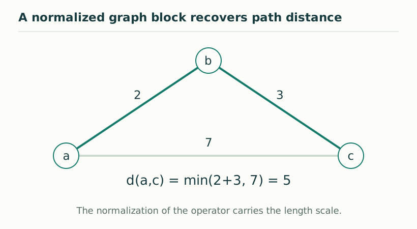
Figure 1. A normalized graph block recovers path distance. For the specified normalized spectral block, the distance equals weighted shortest-path distance. Here the illustrative route a–b–c has length 2+3 = 5, shorter than the direct edge of length 7. View full size ↗
03Compute a local heat dimension
Differentiate the finite sum exactly to obtain d_M(σ)=2σ[Σ|n|²e^(−σ|n|²)]/[Σe^(−σ|n|²)]. At very small σ, all finite modes contribute almost equally and d_M tends to zero. At very large σ, the zero mode dominates and the slope again tends to zero. A plateau near three can occur only in an intermediate window where neither cutoff nor finite-volume saturation dominates. Its stability as M increases is more informative than a single attractive plot.
d_M(σ)=2σ Σ|n|²e^(−σ|n|²)/Σe^(−σ|n|²)
04Check the first counts by hand
At Λ=1 the allowed integer points are the origin and six unit-axis neighbours: seven points, or fourteen with multiplicity two. At Λ=2 there are thirty-three points, giving sixty-six. These small cases are useful implementation checks. They also demonstrate that a stepwise finite count is not exactly proportional to Λ³ at each radius. A meaningful asymptotic fit requires a range containing many shells and remaining below the regulator boundary.
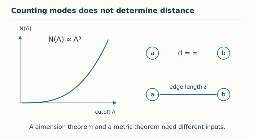
Figure 2. Counting modes does not determine distance. Spectral growth concerns how many modes lie below a cutoff. Distance concerns how observables vary under a normalized operator. The draft gives explicit examples in which the former is finite-dimensional while diagonal-state distances are infinite. View full size ↗
05Add an independent distance experiment
On the same vertex box, build the normalized nearest-neighbour graph block and calculate distances between selected evaluation states. Unit-edge distances are Manhattan distances, while the diagonal number operator alone gives infinite distances in the diagonal sector. The comparison separates two diagnostics that can share labels but probe different structure. For SMM/DTT this finite benchmark is a disciplined development tool: it can verify operator algebra and expose regulator dependence before physical claims are made. It cannot select the microscopic source law, prove a continuum limit or establish Lorentzian propagation from the plotted plateau alone.
06The derivative formula avoids numerical artefacts
A finite-difference derivative of a noisy log heat trace can create spurious plateaus. In this finite model the analytic derivative of the same sum is available, so it should be used as the primary diagnostic and compared with numerical differentiation only as a check. Regulator convergence should vary M while holding physical frequency or length calibration fixed. Rescaling axes separately for each plot can otherwise manufacture an apparent common window. These elementary checks make the numerical exercise useful for SMM/DTT: the calculation becomes a transparent test of a specified operator instead of a visual confirmation of a desired dimension.
07Three diagnostics with different jobs
Spectral counting measures how the number of modes grows with frequency. A commutator seminorm measures which observables can vary between states while remaining Lipschitz bounded. An operational calibration connects these mathematical states and scales to actual records, distances and clocks. None of the three substitutes for the others. A compact auxiliary operator can have a clear counting exponent and nevertheless give infinite distances between selected localized states. Likewise a finite graph can have an exact distance without proving a smooth manifold limit or Lorentzian dynamics. Keeping these tests separate makes the reconstruction more informative and prevents a numerical plateau from being mistaken for complete spatial emergence.
Operator normalization is physical data once a spectral construction is used for measurement. Replacing D by aD multiplies its eigenvalues by a but divides its Connes distances by |a|. The counting exponent can remain unchanged while all calibrated lengths change. Likewise a bounded finite multiplicity changes a leading counting coefficient without changing its exponent. A proposed temporal explanation of geometry should therefore state both dimensionless structural results and dimensional calibrations. Agreement of an exponent with three is useful, but it cannot fix a ruler, a clock or their conversion by itself.
KEEP THE CONNECTION
Key ideas
Finite heat dimensions have cutoff and saturation regimes.
Small exact counts provide useful implementation checks.
Distance should be computed independently on the same record set.
Scope of the argument. Finite benchmark of a supplied spectral model; numerical plateaus are not proofs of continuum emergence.
Sources & further reading
dual_temporal_spectral_triples_v3.pdf — working draftpp. 15–16, §§8–9
Source editions and catalogue entries
Working manuscript
Complex-Time Spectral Triples and the Separation of Spectral Dimension from Metric Distance
Working manuscript. Article-level references identify the consulted sections and the scope of the interpretation. No public URL was supplied for this exact manuscript version.